Spanish
  Chinese
  Russian
  German
  French
  Japanese
  Portuguese
  Hindi
Hindi Case Report, Geoinfor Geostat An Overview Vol: 12 Issue: 6
The Influence of Secondary Data Integration on Multiple Point Geo-Statistical Simulation: A Case Study in the Upper Salzach Valley, Austria
Carmen Jandrisevits* and Robert Marschallinger
1Department of Geoinformatics, University of Salzburg, Salzburg, Austria
*Corresponding Author: Carmen Jandrisevits,
Department of Geoinformatics, University of
Salzburg, Salzburg, Austria
E-mail: carmen.jandrisevits@stud.plus.ac.at
Received date: 10 November, 2024, Manuscript No. GIGS-24-152146;
Editor Assigned date: 12 November, 2024, PreQC No. GIGS-24-152146 (PQ);
Reviewed date: 26 November, 2024, QC No. GIGS-24-152146;
Revised date: 03 December, 2024, Manuscript No. GIGS-24-152146 (R);
Published date: 10 December, 2024, DOI: 10 .4172/2327-4581.1000421.
Citation: Jandrisevits C, Marschallinger R (2024) The Influence of Secondary Data Integration on Multiple Point Geo-Statistical Simulation: A Case Study in the Upper Salzach Valley, Austria. Geoinfor Geostat An Overview.12:6.
Abstract
Multiple-point geostatistical simulation has recently become popular in stochastic hydrogeology, primarily because of its capability to derive geologically reasonable patterns and multivariate distributions from a training image and conditioning training image data to multiple hard and soft data sources. This article resents, evaluates and contrasts the results of using multiplepoint geostatistical simulation for producing geologically realistic models of a Quaternary inner-alpine aquifer. Borehole data, expert-designed geological profiles and training image data were subject to conditional simulation with the Single Normal Equation Simulation (SNESIM) algorithm, one of the most widely used Matrix Product State (MPS) algorithms. The sensitivity of model predictions to the training image and hard as well as soft data input was evaluated. Modeling results indicate that soft conditioning in MPS is a convenient and efficient way for integrating secondary data such as geological expert drawings.
Keywords: Multiple point statistics; Secondary data integration; Aquifer heterogeneity; Quaternary over-deepened alpine basin
Introduction
Aquifer heterogeneity poses challenges to hydrogeological modeling. Due to limited available data, it is essential to integrate all relevant, usually multi-source information in order to reduce the uncertainty in aquifer models and flow predictions. Various geostatistical modeling/simulation approaches have been developed over the past 50 years to assess spatial uncertainty due to interpolation or simulation of observed input variables. In hydrology, variogram based two-point geostatistics and multiple-point geostatistics have been widely used to describe subsurface heterogeneity [1-3]. Twopoint geostatistics have limitations in reproducing the complex curvilinear shapes encountered in sediment associations like Quaternary aquifers. Instead of using mere two-point statistics from a variogram model, the MPS approach borrows multiple-point statistics from a Training Image (TI), which can be regarded as a conceptual model of the involved geological structures. Initially, MPS algorithms generated geologically realistic realizations by using the TI to obtain conditional probabilities needed in a stochastic simulation framework [2]. More recent pattern-based geostatistical algorithms attempt to improve accuracy and efficiency of TI pattern reproduction by abstracting TI contents into a pattern database. Sequential simulation is then carried out by selecting the most probable pattern chunks from this database and pasting them onto the simulation grid. The MPS algorithm SNESIM (Single Normal Equation Simulation), which uses a categorical variable TI, was proposed by [3]. SNESIM enables two-dimensional (2D) or three-dimensional (3D) simulation, necessitating a 2D or 3D TI. The construction of a 3D TI for MPS is not straightforward, since most geological investigations-with the exception of 3D geophysics-do not deliver volumetric data but merely surface-related observations like mapping, profile sections, or 3D point observations such as borehole data [4]. Currently, objectbased simulation is popular for creating 3D TIs since TIs need not be conditional to data, but must only represent the typical geometric shapes of involved geo-objects and the spatial relationships between them [5,6]. MPS can be conditioned to hard data like drillings and to soft data such as geophysical data or expert-derived geological sections. Another advantage of MPS is the ability to incorporate multiple sources of data [7-10]. This paper highlights reproducing the heterogeneity of aquifer sediments by means of the SNESIM algorithm. SNESIM was used to model the shallow aquifer structures of a Quaternary over-deepened alpine basin in the Upper Salzach Valley, Austria. Aquifer models were simulated conditioned to hard data from drillings, but also fully conditional realizations, both with hard and soft data, were run. Expert-created geological sketches served as secondary soft data. The influence of secondary data integration on simulation results was evaluated.
Study area and database
The study area is located in the Upper Salzach valley, Zell region and covers an area of 3 km × 2 km (Figure 1). Geological investigation suggests a highly heterogeneous sedimentary infill of fluvial and lacustrine origin with variable vertical and lateral extents indicating diversified aquifer structures. Investigation data are sparse and comprise drillings, 2D geophysical exploration data and geological sketches. There are 56 drillings with variable drilling depths from 5 m-50 m, whereby only 10 groundwater wells reach a depth of 50 m. Regarding assumed hydrological parameters, sediments were categorized in three classes: Gravel, Sand and Silt/ Clay. Borehole descriptions and geological sketches were categorized accordingly. Input data were discretized and simulated into a 3D grid with SNESIM. For a subarea (200 m × 200 m), a grid dimension of 1 m × 1 m × 0.2 m was chosen. The subarea was discretized with a cell size of 15 m × 15 m × 0.5 m.

Figure 1: Location of the study area and the investigation subarea in the upper Salzach valley drained by the Salzach river in Austria. Orthoimagery and Digital Elevation Model were obtained from an internet source.
Case Representation
The theory of Multiple-Point geostatistics was developed over the past three decades as a powerful method for deriving realistic geostatistical models with complex structures. Today, MPS is widely used in a variety of geoscience fields, including but not limited to reservoir modeling [11-12], hydrology and geological modeling [13-15].
Using the single normal equation simulation (SNESIM) algorithm for multiple point statistical (MPS) simulation
The primary advantage of MPS is its capability to capture multiplepoint based structure information instead of using two-point-based statistics yielded by variography [16]. The database from which the structural information is retrieved is referred to as TI. In the present context, a TI is any categorical 2D or 3D image which contains the geological conceptualization of the target variable [17]. It is not a subsurface model itself, but a quantitative conceptual depiction of it. The user chooses the TI based on his/her prior understanding of the local hydrogeological system. The TI does not necessarily provide locally accurate information; i.e., there is no need to contain the actual georeferenced positions of the hydrostratigraphic architecture, just the general patterns. The TI needs to reflect a prior geological or structural concept containing geologically realistic and relevant information, however [12,18]. It is a tool to identify the dominant patterns and their variation. TI production is a most important stage of the simulation process since the output critically depends on it. A TI can be produced using different methods and available data sources. 19. Comunian A et al., pointed out that while a 3D TI is necessary for 3D MPS simulation, it is not trivial to generate a 3D TI since geological observations generally only provide 2D information [19]. Hence, 3D simulation is an important challenge for MPS [4]. Okabe H et al., as well as Okabe H et al., generated 3D TI realizations by applying information from lateral 2D images on orthogonal directions [11,20]. Coz et al., built a 3D TI by successively replicating a single 2D TI. These “copy and paste” methods are simple but certain assumptions need to be invoked [13]. Other methods include complicated statistical simulations such as described by Comunian et al., [21]. They used probability aggregation approaches to retrieve statistical information from 2D TIs which subsequently were applied to simulate a 3D TI. Maharaja A et al., proposed a simple object based algorithm, TI generator, to generate parametric images [22]. However, an image purely generated by stochastic methods lacks evidence from geological observations and its application in MPS can be questioned. He et al., generated two kinds of 3D training images; One TI was generated by direct conversion from SkyTEM data and the other training image was developed by the TI generator implemented in SGeMS [23]. Hoyer et al., constructed a 3D TI based on the well-known geology and used different types of input data for MPS simulation. In this study, the object-based TI generator Tetris was used for Training Image production [14,24]. The SNESIM algorithm combines the flexibility of pixel-based algorithms and the ability to reproduce crisp shapes of object-based algorithms. Of note, SNESIM simulations can be run on standard hardware with reasonable computing power. The critical step of sequential simulation is the Conditional Probability Distribution Function (CPDF). The SNESIM algorithm is based on the following equation:
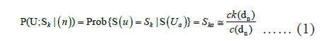
This solution is achieved by scanning a TI by a template consisting of n+1 nodes that is centered at location U, the values c (dn) and ck (dn) are recorded while scanning the TI. dn denotes the data event of all n surrounding nodes. c (dn) denotes the number of replicates of the conditioning data event dn =(S(Ua)=Ska, a=1,···,n) and ck (dn) denotes that among those c (dn) replicates, the number of replicates with the central node U has the value S(U)=Sk. The equation above implies that the probability of state Sk to occur at location 1 with n neighbor data is equal to the training proportion ck (dn)/c (dn). These training probability values are stored in a search tree a prior to simulation. With the possession of cpdf, the sequential simulation paradigm is used in stochastic simulation [25]. The hard data is first assigned to the closest grid nodes and all the unknown grid points are visited once and only once in a random path. At each unknown location U, the recorded cpdf corresponding to actually present hard conditioning data event is retrieved and is used to draw the simulated value S at this location.
Training Image (TI) construction
Different scenarios of MPS simulations were designed with different combinations of TI and soft data to provide evidence of MPS applicability. The TI includes geometries of the three classified sediment groups and inherently contains erosion relations. The TI size is 127 m × 67 m × 4.4 m (X × Y × Z) with a spatial resolution of 1 m × 1 m × 0.2 m. Figure 2 is an oblique, semi- transparent view of the TI, exposing its internal structure: A matrix of sand sediments (orange color) holds intercalated silt-clay ponds (green color), all cut by gravel channels (yellow color) (Figure 2).

Figure 2: 3D view of the training image containing. Note: a) gravel ( ), (
), ( ) and silt/clay (
 ) sediments; b) visualizing only gravel channels
(); c) visualizing only silt/clay ponds ().
) sediments; b) visualizing only gravel channels
(); c) visualizing only silt/clay ponds ().
Soft data conditioning
Another advantage of MPS is the ability to incorporate multiple sources of data [8,9,26]. Comunian A et al., concluded that the sensitivity of the model predictions to the training image is a central topic of further research [21]. Accompanying TI information, soft data (e.g., geophysical data, geological sketches) can be included for constraining MPS simulations, resulting in realizations that also honor real-world regional geology. Soft data or secondary data relate to indirect information on the distribution of geological facies. Typical soft data include geophysical data such as seismics or geoelectrics. The integration of soft data for constraining the simulations is achieved by the so-called tau model. Here, the continuous soft data variable needs to be translated into a probability grid, describing the probability of finding a given geological unit based on the secondary data [27]. In order to guarantee the reproduction of geological patterns at all scales, SNESIM uses the multiple-grid formulation, presented by [28]. To enable integration in SNESIM, soft data first have to be converted into facies probability data. If n is the facies indicator value at location u, then P(A) is the facies global proportion or prior probability in Bayesian statistical terms. B infers to data event from training image. Then P(S(U)=Sk|dn)) in Eq.1 can be rewritten as PA|B. Let C represent the additional soft information, then PA|C denotes the probability derived from soft data. Derived a Bayesianbased model of integrating PA|B and PA|C [29].
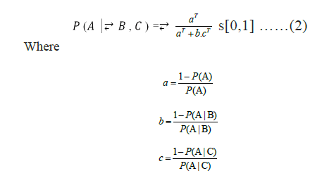
The parameter τ is used to adjust the contribution of soft information C. τ=1 indicates independence of contribution of data C from data B. For τ=0, the soft information is ignored, while for τ > 1, the influence of soft data C is increased and it is decreased for τ < 1. The two weights τ1 and τ2 account for information redundancy between the closest prototype prob(u) and the local soft data event sdev(u), respectively. The default values are τ1=τ2=1 [30,31].
Geological profile construction
In this study, geological expert knowledge was combined with borehole data to draw 2D geological sketches which were later incorporated as soft data in SNESIM. Based on classified drilling logs from nine drill holes within the zone of the subarea, a geologically possible and probable scenario of the sedimentary structure was developed. The scenario represents a situation in a typical foreland region of a melting glacier. For the scenario, three cross sections in SW-NE-direction (A-A’, C-C’, D-D’) and one in SE-NW-direction (B-B’) were constructed between drill holes, obeying consistency at the intercept points of cross sections. Figure 3 gives the location of the cross sections.

Figure 3: Location of drillings (enlarged in the horizontal direction) and constructed cross-sections (gravel (), sand () and silt/clay ()).
For consistency, identical categorization was applied to crosssections as to hard data from drilling logs: Three classes of lithologies were distinguished-gravel (yellow), sand (orange) and silt and clay (green). The top-most meters in the southern, southwestern and central parts of the study area are dominated by sedimentation of silt and clay due to a lacustrine environment as the youngest sedimentation process. In the north and northeast, sandy layers dominate the uppermost horizons and delineate the lake to the north. In the middle part (one to seven meters below the surface), the dominating component is sand, interspersed by layers of clay and gravel.
This indicates generally moderate flow velocities with seasonal variations (snowmelt in spring, low flow conditions in autumn and winter). The deepest part is dominated by gravel in the central, southern and eastern areas, while sand is the most frequent component in the western and northern areas. This can be interpreted as a flow channel crossing the study area in the south and southeast. Figure 4 shows the geological cross-sections.

Figure 4: Schematic representation of geological cross-sections. Note: a) A’; b) B’; c) C’; d) D’ (gravel (), sand () and silt/clay ()).
Above 2D sections were constructed with CAD software and exported as ASCII files. Individual ASCII ASCII files were combined in one GSlib file which facilitates the import in SGeMS v2 [32].
Servosystem
The servosystem correction attracts the running simulated marginal probability toward the target probability at each moment of the sequential simulation process. Let Pc(A) be the probability of event A, calculated using the existing and simulated points before simulating point x. For simulating point x, instead of using the conditional probability P(AǀB) (eventually updated using the above Bayesian formula), a correction toward the target probability P × (A) is introduced by using

The degree of correction increases with the value of λ. P(A|B) may not necessarily honor the order relations. Similar to the sequential indicator simulation, a correction of order relations is applied to P(A|B) before simulation. Shows that increasing the value of λ can make the global statistics of a simulation closer to the target statistics, but at the cost of losing geometric features of the TI. This is because the marginal probability and the MP statistics are not decoupled. It is recommended that the target statistics should not be too different from that of the TI. This requires building training images that are representative both in terms of geometric features and global statistics [9].
Single Normal Equation Simulation (SNESIM) parameterization
Different scenarios of MPS simulations were designed with different combinations of TI and soft data to provide evidence of MPS applicability. The MPS simulation grid is 254 m × 134 m × 17 m (xyz), with xyz grid cell dimensions of 1 m × 1 m × 0.2 m, including the following three categories: Quaternary gravel, Quaternary sand and Quaternary silt/clay. For soft data inclusion, the SNESIM algorithm requires probability data calibrated from soft data. To infer 3D probability maps of a particular facies' occurrence at a specific grid point (voxel array), we used Indicator Kriging on one hand (F and Sequential Indicator Simulation on the other hand (Figures 5 and 6). The probability of facies occurrence ranges from 0 (lowest probability, blue color) to 1 (highest probability, red color).

Figure 5: Probability map for mentioned ones. Note: a) Gravel; b) Sand and c) Silt/clay facies obtained by Indicator Kriging (0=lowest
probability ( ) to 1=highest probability (
 )).
)).

Figure 6: Probability map for mentioned ones. Note: a) Gravel; b) Sand c) Silt/clay facies obtained by Sequential Indicator Simulation
(0=lowest probability () to 1=highest probability ()).
Results and Discussion
This section presents the results of different simulations conditioned to hard and soft data. Five different models with varying Tau values and servosystem factor values were analyzed. For a better comparison of the different models, 3D views of model cuts and tables including facies distribution, as well as histograms, are depicted. In the first approach, the most traditional one, borehole data were used as hard conditioning. One SNESIM realization conditioned only to hard data is shown in Figure 7. Here, SNESIM simulation effectively reproduces the depositional patterns provided by the TI and facies distribution around drillings, as well as facies connectivity distant from drillings, are simulated in a sedimentologically consistent manner (Figure 7).

Figure 7: Location of drillings. Note: a) SNESIM realization with hard data only conditioning (xyz voxel size: 1 m × 1 m × 0.2 m); (b) Same
as Figure 7a, but sliced at z=745m to visualize internal structure; c) Histogram of the SNESIM realization in Figure 7a (gravel (), sand ()
and silt/clay ()).
The uncertainty in geological simulation models will decrease with additional data sources; however, it is not easy to reconcile various data because they have varying scales and spatial coverage. Secondary data typically have a larger scale than the modeling scale. In a second step, the impact of secondary data integration on simulation results in the investigation area was analyzed. Incorporating probability maps into SNESIM, a further set of facies realizations was generated. The histogram of soft data is shown in Figure 8. These realizations are conditioned not only to drill logs but also to geological soft data (derived from geological sections in Figure 9).

Figure 8: Histogram of soft data (cross sections).

Figure 9: Location of drillings. Note: a) SNESIM realization with hard and soft data conditioning with τ1=τ2=1, servosystem factor=0.9 (voxel size: 1 m × 1 m × 0.2 m); b) same as Figure 9a, but sliced at z=745m to visualize internal structure; c) related histogram of the SNESIM realization in Figure 9a.
The SNESIM realization in Figure 9a, equal weights (τ1=τ2=1) were assigned to the soft data and training image. The servosystem factor was set to 0.9, the same as in the SNESIM realization conditioned only to hard data (Figure 7). The gravel bodies appear in a patchy, discontinuous form and silt/clay deposits are smaller compared to the model conditioned only to hard data. In Figure 10, different τ-values (τ1=1, τ2=0.5) were used, while the value of the servosystem factor was kept at 0.9. Reducing the weight of the secondary (soft) data, the channel structure of gravel facies is still visible in realization Figure 10, but with a shorter length and smaller width compared to the channels in the model without soft data conditioning. For the simulation of the model in Figure 11, the servosystem factor is set to 0 and the weights (τ1=τ2=1) were assumed to be equal. In the realization Figure 11, the channel structures have the highest sinuosity compared to previous SNESIM simulation models. Experimental results show that the structures simulated using both soft and hard data are most similar to those of the training image when IK is used for soft data input. When integrating secondary data first, it is important to properly account for data redundancy, which represents how closely secondary data are related to the primary data [33]. In the third step, facies in the 2D geological profiles were used as input for SISIM and the obtained 3D probability models were used as soft conditioning for SNESIM. The SISIM probability model input shown in Figure 6 for soft data conditioning with τ1=τ2=1, servosystem factor=0.9 (Figure 12). Here, the geobodies of the sediment facies appear geologically unrealistic.

Figure 10: Location of drillings. Note: a) SNESIM realization with hard and soft data conditioning with τ1=1, τ2=0.5, servosystem factor=0.9 (voxel size: 1 m × 1 m × 0.2 m); b) same as Figure 10a, but sliced at z=745 m to visualize internal structure; c) related histogram of the SNESIM realization in Figure 10a.

Figure 11: Location of drillings. Note: a) SNESIM realization with hard and soft data conditioning with τ1=τ2=1, servosystem factor=0 (voxel size: 1 m × 1 m × 0.2 m); b) same as Figure 11a, but sliced at z=745 m to visualize internal structure; c) related histogram of the SNESIM realization in Figure 11a.

Figure 12: Location of drillings. Note: a) SNESIM realization with hard and soft data conditioning with τ1=τ2=1, servosystem factor=0 (voxel size: 1 m × 1 m × 0.2 m); b) same as Figure 12a, but sliced at z=745 m to visualize internal structure; c) related histogram of the SNESIM realization in Figure 12a.
Table 1 below depicts the facies proportions of input data and simulation realizations. According to hard data and soft data, the sand facies have the highest proportion, the gravel facies have the second highest proportion and the silt/clay facies have the smallest proportion (exception: Simulation 6). The gravel facies have the highest deviation (12 percent) compared to the hard data and soft data input.
| No. | Type of input data or simulation | Gravel (prop.) | Sand (prop.) | Silt/ Clay (prop.) |
|---|---|---|---|---|
| 1 | Hard data | 0,40 | 0,45 | 0,15 |
| 2 | Soft data-cross sections | 0,28 | 0,52 | 0,20 |
| 3 | Snesim-simulation with hard data | 0,40 | 0,45 | 0,16 |
| 4 | Snesim-simulation with hard data and soft data (calculated by means of IK) with τ1=τ2=1 and servosytemfactor=0.9 | 0,38 | 0,46 | 0,16 |
| 5 | Snesim-simulation with hard data and soft data (calculated by means of IK) with τ1=1 τ2 = 0.5 and servosytemfactor=0.9 | 0,28 | 0,53 | 0,20 |
| 6 | Snesim - simulation with hard data and soft data (calculated by means of IK) with τ1=τ2=1 and servosystemfactor=0 | 0,48 | 0,35 | 0,17 |
| 7 | Snesim-simulation with hard data and soft data (calculated by means of SISIM) with τ1=τ2=1 and servosytemfactor=0.9 | 0,34 | 0,52 | 0,14 |
Table 1: Facies proportions of data and simulation models.
This study suggests that soft conditioning in MPS is a convenient and efficient way of integrating secondary data, such as 2-D geological profiles, but over-conditioning has to be avoided. It can result in realizations that both honor the input statistics and resemble real geology.
Conclusion
This paper described and applied multiple-point geostatistical simulation of a sediment association in a Quaternary aquifer, using different combinations and weightings of hard data (drilling logs) and soft data (derived from expert-designed geological cross sections). The stochastic simulations were conducted using the SNESIM algorithm as implemented in SGeMS. The training image was constructed with a training image generator. Multiple Point Geostatistical Simulation is a flexible and efficient method for building an ensemble of equally probable, geologically realistic realizations. This is especially important when only sparse primary data are available in complex and heterogeneous geological areas. For practitioners without a deeper understanding of the details of a given MPS method, simulation can be difficult to handle. Fine-tuning the weights of hard and soft data, or the number of candidate patterns in the pool, patch sizes, overlap region width, or weighting matrices can be challenging. To verify the reliability of the proposed geological sediment facies simulations in this study, groundwater flow modeling should be addressed in future research.
References
- Deutsch CV, Journel AG (1992) GSLIB Geostatistical Software Library and User’s Guide. New York: Oxford University Press.
- Guardino F, Srivastava RM(1993) Multivariate geostatistics: Beyond bivariate moments. Geostatistics Troia 13(3):41-44.
- Strebelle S(2000) Sequential simulation drawing structures from training images. PhD dissertation, Stanford University, Stanford, California.
- Huysmans M, Dassargues A(2009) Application of multiple-point geostatistics on modeling groundwater flow and transport in a cross-bedded aquifer. Hydrogeol 17(8):1901–11.
- Boucher A (2011) Strategies for Modeling with Multiple-Point Simulation Algorithms. Gussow Geoscience Conference Banff, Alberta.
- Marschallinger R, Orsi G, Burger U, Gerhard P. Multiple-point geostatistics for the 3D modeling of geological formations.
- Strebelle S(2002) Conditional simulation of complex geological structures using multiple-point statistics. Math Geol 34(1):1–21.
- Strebelle SB( 2006) Sequential simulation for modeling geological structures from training images. Model Geostat 139-49.
- Hu L, Chugunova T. Multiple-point geostatistics for modeling subsurface de Bonet JS. Multiresolution sampling procedure for analysis and synthesis heterogeneity: A comprehensive review. Water Resour Res 20:44.
- Hansen TM, Vu LT, Cordua KS (2018) Multiple-point statistical simulation and uncertain conditional data. Comput Geosci114:1-10.
- Okabe H, Blunt MJ(2005) Pore space reconstruction using multiple-point statistics. J Petrol Sci Eng 46:121–37.
- Strebelle S, Journel AG( 2001) Reservoir Modeling Using Multiple-Point Statistics. Society of Petroleum Engineers Annual Technical Conference and Exhibition New Orleans, LA.
- Coz ML, Genthon P, Adler PM (2011) Multiple-point statistics for modeling facies heterogeneities in a porous medium: The Komadugu-Yobe Alluvium, Lake Chad Basin. Math Geosci 43(7):861–78.
- Hoyer AS, Vignoli G, Hansen TM, Vu LT, Keefer DA, et al. (2017) Multiple-point statistical simulation for hydrogeological models: 3D training image development and conditioning strategies. Hydrol Earth Syst Sci 21:6069–89.
- De Iaco S, Maggio S (2011) Validation techniques for geological patterns simulations based on variogram and multiple-point statistics. Math Geosci 43:483–500.
- Journel AG(2005) Beyond covariance: The advent of multiple-point geostatistics. Springer. 225: 33.
- Mariethoz G, Caers J. Multiple-Point Geostatistics: Stochastic Modeling With Training Images. John Wiley & Sons.
- Journel AG, Zhang T(2006) The necessity of a multiple-point prior model. Math Geol 38(5):591–610.
- Comunian A, Renard P, Straubhaar J, Bayer P (2011) Three-dimensional high-resolution fluvio-glacial aquifer analog, part 2: Geostatistical modeling. J Hydrol 405:10–23.
- Okabe H, Blunt MJ(2007) Pore space reconstruction of vuggy carbonates using microtomography and multiple-point statistics. Water Resour Res 43: 12.
- Comunian A, Renard P, Straubhaar J (2012) 3D multiple-point statistics simulation using 2D training images. Comput Geosci 40:49–65.
- Maharaja A (2008) TiGenerator: Object-based training image generator. Comput Geosci 34:1753–61.
- He X, Sonnenborg T, Jorgensen F, Jensen KH(2014) The effect of training image and secondary data integration with multiple-point geostatistics in groundwater modelling. Hydrol Earth Syst Sci 18(8):2943–54.
- Boucher A, Gupta R, Caers J, Satija A (2010) Tetris: A Training Image Generator For SGEMs. Proceedings of the 23rd SCRF Annual Affiliates Meeting.
- Goovaerts P(1997) Geostatistics for Natural Resource Evaluation. Oxford University Press.
- Liu Y (2006). Using the Snesim program for multiple-point statistical simulation Comput Geosci 32(10):1544–63.
- Barfod AAS, Møller I, Christiansen AV, Høyer AS, Hoffimann J, et al. (2018) Hydrostratigraphic modeling using multiple-point statistics and airborne transient electromagnetic methods. Hydrol Earth Syst Sci 22:3351-73.
- Tran T (1994) Improving variogram reproduction on dense simulation grids .Comput Geosci 25(7):1161–8.
- Journel AG(2002) Combining knowledge from diverse sources: An alternative to traditional data independence hypotheses. Math Geol 34(5):573–96.
- Krishnan S. Combining Diverse and Partially Redundant Information in the Earth Sciences.
- Liu Y, Harding A, Gilbert R, Journel AG (2004) A workflow for multiple-point geostatistical simulation. Quant Geol Geostat 245: 54.
- Remy N, Boucher A, Wu J (2009) Applied Geostatistics with SGeMS: A User’s Guide. Cambridge University Press.
- Hong S, Deutsch CV (2009) On Secondary Data Integration. Annual Report 11(101):1.