Spanish
  Chinese
  Russian
  German
  French
  Japanese
  Portuguese
  Hindi
Hindi Research Article, Geoinfor Geostat An Overview Vol: 12 Issue: 4
Seismic Nowcasting: A Systemic Artificial Neural Network Predictive Model
Anastasios N. Bikos*
Department of Computer Engineering and Informatics, University of Patras, Patras, Greece
*Corresponding Author: Anastasios N. Bikos,
Department of Computer Engineering and
Informatics, University of Patras, Patras,
Greece;
E-mail: mpikos@ceid.upatras.gr
Received date: 22 August, 2024, Manuscript No. GIGS-24-146155;
Editor Assigned date: 26 August, 2024, PreQC No. GIGS-24-146155(PQ);
Reviewed date: 09 September, 2024, QC No. GIGS-24-146155;
Revised date: 16 September, 2024, Manuscript No. GIGS-24-146155(R);
Published date: 23 September, 2024, DOI: 10 .4172/2327-4581.1000402.
Citation: Bikos AN. Seismic Nowcasting: A Systemic Artificial Neural Network Predictive Model. Geoinfor Geostat An Overview.12:4
Abstract
A contemporary technique for calculating seismic risk is Earthquake Nowcasting (EN), which analyzes the progression of the Earthquake (EQ) cycle in fault systems. "natural time" is a novel idea of time that serves as the foundation for EN assessment. The Earthquake Potential Score (EPS), which has been discovered to have practical uses regionally and worldwide, is a unique tool that EN uses to predict seismic risk. For the estimation of the EPS for the occurrences with the highest magnitude among these applications, since 2021 we have concentrated on Greece territory, applying sophisticated Artificial Intelligence (AI) algorithms, both wise (semi) supervised and unsupervised models, along with a customized dynamic sliding window technique that performs as a stochastic filter able to fine-tune the geoseismic occurrences. Long and Short Term Memory (LSTM) neural networks, random forests and clustering (geospatial) models are three machine learning techniques that are particularly good at finding patterns in vast databases and may be used to improve earthquake prediction performance. This study attempts to forecast whether practical machine learning and AI/Game-theoretic-based approaches can help predict big earthquakes and the normal future seismic cycle for 6-12 months. Specifically, we focus on answering two questions for a given region: (1) Can a significant earthquake, say one of magnitude ≥6.0, occur in the upcoming year? (2) What is the most significant earthquake magnitude predicted in the upcoming year and with which exact Geographic Coordinates (GCS)? Our results are pretty promising and project a high precision accuracy score (≥98%) for seismic nowcasting in terms of four predictive parameters: The approximate (a) latitude (b) longitude (c) focal depth and (d) magnitude of the phenomena.
Keywords
Earthquake nowcasting; Machine learning; Game theory; Clustering; Seismic risk; Statistical methods; Long shortterm memory neural network.
Abbreviation
ANN: Artificial Neural Network; LSTM: Long Short-Term Memory; SW: Sliding Window; XGBoost: eXtreme Gradient Boosting; EQ: Earthquake.
Introduction
One of the worst natural disasters on the planet, earthquakes frequently result in significant loss for the human race. As a result, it is imperative to foresee when and where they will occur, although doing so is difficult due to their inherent randomness [1].
The earthquake prediction methods that are nowadays commonly used can be categorized into four groups according to [2]. The first two strategies, namely:
• Mathematical tools like FDL and
• Precursor-based techniques that retrieve geographic features such as seismic anomalies, cloud images and animal behavior were well liked when there was a shortage of earthquake data [3-6].
Then as more and more earthquakes produced larger datasets, machine learning techniques entered the picture. Moustra et al., used an artificial neural network, one of them, to predict an earthquake in 2011 [7]. The model accuracy was about 70%, which was not very good then. It was determined from the research that fewer attributes in the dataset, as well as the class imbalance, led to unsatisfying results.
Finally, deep learning techniques have recently been used to forecast earthquakes. A Deep Neural Network (DNN) model that evaluated earthquake magnitudes that will occur within the next seven days using a newly introduced parameter fault density (based on the concept of spatial effect) was tested by Yousefzadeh et al., [8]. DNN performed better than other machine learning models, with a test accuracy of about 79% on magnitudes greater than 8. To detect epicenters of earthquakes that occurred in the past two months, Ruiz et al., developed a network called the Graph Convolutional Recurrent Neural Network (GCRNN) by combining the properties of Convolutional Neural Networks (CNN) and recurrent neural networks [9]. GCRNN used convolutional filters to maintain the independence of the trained parameter count from the input time sequences. For both the 30-second and 60-second waves, GCRNN achieved an accuracy of about 33% with fewer characteristics being taken into account. In addition, Wang et al., used a variation in Long-Short- Term Memory (LSTM) of the recurrent neural network to learn the temporal-spatial dependencies of seismic signals and consequently forecast earthquakes [2]. Although they only used seismic data from the previous year as input, the precision was about 75%. Kavianpour et al., suggested a CNN-LSTM hybrid network to learn the spatialtemporal dependencies of earthquake signals [10]. They used the total number of earthquakes that occurred in a single month between 1966 and 2021 as their input to evaluate the effectiveness of the model in nine regions of the Chinese mainland. They also included other earthquake-related factors, such as latitude and longitude. They compared the results of several models, including MLP and SVM and found that CNN-LSTM scored the highest.
In Xiangyu et al., the author(s) focuses on predicting an earthquake in the next 30 seconds [11]. Even though a long-term prediction’s outcome is likely erroneous (not accurate to a single day), 30 seconds allows individuals enough time to react and prevent an unthinkable tragedy. They finally implemented different time series models (vanilla RNN, LSTM and Bi-LSTM) compared to each other in the same study question.
More recent research studies outline alternative neural network technologies. In recent years, neural networks, including LSTM and convolution neural networks, have been widely used in the research of time series and magnitude prediction [7,12]. As mentioned earlier, using LSTM networks to record spatio-temporal correlations among earthquakes in various places, the authors of Boucouvalas et., developed a novel method for predicting earthquakes [3]. Their simulation findings show that their strategy performs better than conventional methods. The accuracy of earthquake prediction has been shown to increase by using seismicity indicators as input in machine learning classifiers [13]. The results of using this methodology in four Chilean cities show that reliable forecasts can be made by thoroughly examining how specific parameters should be configured. Asim et al., describes a proposed methodology trained and tested for the Hindu Kush, Chile and Southern California regions [14]. It is based on the computation of seismic indicators and the GPAdaBoost classification. Compared to earlier studies, the prediction results derived for these regions show an improvement. Alvarez et al., explores how Artificial Neural Networks (ANNs) can be used to predict earthquakes [15]. The results of the application of ANNs in Chile and the Iberian Peninsula are presented and the findings are compared with those of other well-known classifiers. Adding a new set of inputs improved all classifiers, but according to the conclusion, the ANN produced the best results of any classifier.
Seven different data sets from three areas have been subjected to a methodology to identify earthquake precursors using clustering, grouping, building a precursor tree, pattern extraction and pattern selection [16]. The results compare favorably to the previous edition in terms of all measured quality metrics. The authors propose that this method could be improved and used to predict earthquakes in other places with various geophysical characteristics.
The authors of Rundle, J et al., employ machine learning techniques to identify signals in a correlation time series that predict significant future earthquakes. Decision thresholds, Receiver Operating Characteristic (ROC) techniques and Shannon information entropy are used to assess overall quality [17]. They anticipate that the deep learning methodology would be more all-encompassing than earlier techniques and will not require guesswork upfront about whether patterns are significant. Finally, their findings in Wang et al., demonstrate that the LSTM technique only provides a rough estimate of earthquake magnitude, whereas the random forest method performs best in categorizing major earthquake occurrences [18]. The author(s) conclude that information from small earthquakes can be used to predict larger earthquakes in the future. Machine learning offers a potential way to improve earthquake prediction.
Research contribution
To technically elaborate and materialize this claim, a study was carried out using four seismic features °N, °E, km, Mag. Based on seismic catalogs from the National Observatory of Athens (NOA), Greece containing the full list (that is, small and large magnitude occurrences) of past earthquake events and for a specific year frame. This input was granted to construct a solicit timescaled “Sliding- Window” (SW) mathematical technique that, if co-deployed with advanced machine learning and game-theoretic algorithms, would significantly impact increasing the future precision accuracy of the earthquake predictability. Additionally, the capability of having architectured a synthesized seismic predictability framework that is capable of endorsing Machine Learning (both (semi)supervised and unsupervised), Game-theory solving models (i.e., OpenAI Gym, which is a toolkit for developing and comparing Reinforcement Learning (RL) algorithms), as well as the adaptation of the SW model in seismic short- term and long-term casting was explored. The research investigation emphasized two important questions.
• Will there be a strong event M 6.0, 7.0, or 8.0 forecasted in the next year among the specific studied geographical region?
• Can we obtain the scientific ability to predict the nearly exact 4-tuple °N, °E, km, Mag output of such a future major event, as well as the (implicit) almost exact time frame of its occurrence?
Proof of methods
Greece is a laboratory for natural seismology because it has the highest seismicity in Europe and statistically produces an earthquake of at least M6.0 almost every year [19-21]. The short repeat time in the area also makes it possible to study changes in regional seismicity rates over “earthquake cycles”. Here, we provide the results of the novel earthquake now casting approach developed by Rundle et al., [22]. With this approach, we counted the number of tiny EQs since the most recent major EQ to determine the region’s current hazard level. The term “natural time,” coined by Varotsos et al., refers to event counting as a unit of “time” as opposed to clock time [23-27]. According to Rundle et al., applying natural time to EQ seismicity offers the following two benefits: In addition, when computing nowcasts, the concept of natural time, which is the number of small EQs, is used as a measure of the accumulation of stress and strain between large EQs in a defined geographic area [22]. First, it is not necessary to declutter aftershocks because natural time is uniformly valid when aftershocks dominate, when background seismicity dominates and when both contribute.
In other words, the use of natural time is the foundation of nowcast. As previously mentioned, there are two benefits to using natural time: first, there is no need to separate the aftershocks from the background seismicity; second, only the natural interevent count statistics are used, as opposed to the seismicity rate, which also takes into account conventional (clock) time. Instead of focusing on recurrent events on particular faults, the nowcasting method defines an “EQ cycle” as the recurring large EQs in a vast seismically active region composed of numerous active faults. Following Pasari et al., we may say that although the concept of “EQ cycle” has been used in numerous earlier seismological investigations, the idea of “natural time” is unique in its properties [28-32].
Estimation of seismic risk in large cities around the world, study of induced seismicity, study of temporal clustering of global EQs, clarification of the role of small EQ bursts in the dynamics associated with large EQs, understanding of the complex dynamics of EQ faults, identification of the current state of the “EQ cycle”, the nowcasting of avalanches [33-37]. The Olami-Fe Here, using the earthquake potential, we examined the greatest events in Greece between 1 January, 2023 and 6 February, 2023 with MW(USGS) 6 (Figure 1 and Table 1), utilizing the Earthquake Potential Score (EPS) [38-41].

Figure 1: Map with the seismic events of “higher” EQs scale within a specific Greece megacity. Large EQ comes from “smaller” events within the circular radius region.
| Actual seismic condition | Predicted seismic condition is positive | Predicted seismic condition is negative |
|---|---|---|
| Positive | True Positive (TP) | False Positive (FP) |
| Negative | False Positive (FP) | True Negative (TN) |
Table 1: Confusion matrix of the binary classification problem.
Natural Time Analysis (NTA), which was discussed in Varotsos et al. and more recently in general, displays the dynamical evolution of a complex system and pinpoints when it hits a critical stage [27,42]. As a result, NTA can play a significant role in foreseeing approaching catastrophic occurrences, such as the emergence of massive EQs [43- 47]. In this regard, it was used in EQ situations in Greece, Japan, the USA, Mexico, the Eastern Mediterranean and globally [48-51]. We observe that NTA allows the insertion of an entropy, S which is a dynamic entropy that demonstrates positivity, concavityand experimental stability for Lesche [52-56]. Recently, EQ research in Japan and Mexico has used complexity metrics based on natural temporal entropy and S itself, with encouraging results [57-61]. In particular, two quantities, which are discussed in the following have recently been stated in the Preface of Varotsos et al. and have emerged through natural time analysis to be important in determining whether and when the critical moment (mainshock, the new phase) is approaching [62-66].
First, let us talk about the order parameter of seismicity K1 [67- 71]. Its value 0.070 indicates when the system reaches the critical stage and its minimum value indicates when the Seismic Electric Signals (SES) activities start [72-76]. The SES amplitude is important because it allows one to estimate the impending mainshock’s magnitude [77-80]. The epicentral area is determined using the station’s SES selectivity map, which records the pertinent SES (using this methodology, a successful prediction for a MW =6.4 EQ that occurred on 8 June 2008 in the Andravida area of Greece was made [44,46,81] .
Second, the entropy change, ΔS under time reversal: its value, when minimized a few months in advance, denotes the beginning of precursory phenomena; as for its fluctuations (when the minimum of ΔS appears), they show a clear increase, denoting the time when preparation of EQ begins, as explained by the physical model that served as the basis for SES research [79].
The MW = 9.0 Tohoku EQ on 11 March, 2011 which was the largest event ever recorded in Japan and the MW=8.2 Chiapas EQ on 7 September, 2017 which was the largest EQ in Mexico in more than a century, were used to study precursory phenomena before the two subsequent major EQs.
Datasets and feature engineering
The seismic input catalog used in this research study was provided by the Greece National Observatory of Athens (NOA) and includes earthquake events of magnitude greater than 2.0 in the Greek geographic region between 1950 and 2024. Using feature engineering, several statistical principles were used to create seismic activity parameters for a specific experimentation trial set; rather than using the original seismic catalog, these parameters obtained from it were utilized as input features for earthquake prediction. Another supplementary global public catalog we co-utilized as a proof-of-concept and to minimize historical accuracy metrics loss was the USGS. Specifically, the ANSS Comprehensive Earthquake Catalog (ComCat) includes products generated by contributing seismic networks, such as moment tensor solutions, macroseismic information, tectonic summaries and maps, in addition to earthquake source parameters, such as hypocenters, magnitudes, phase picks and amplitudes. Numerous seismic properties obtained from earthquake catalogs have been shown in previous studies to be useful in earthquake prediction.
The number and maximum/mean magnitude of previous earthquakes, the release of seismic energy, the magnitude deficit, the fluctuations of seismic rates and the amount of time since the last significant earthquake 6 are some of these characteristics. Other elements include a value a value for b in the Gutenberg-Richter (GR) law. Typical related research work seismic features also include the probability of an earthquake occurring, the divergence from the Gutenberg-Richter rule and the standard deviation of the estimated b value. The GR property, which describes the fractal and/or power law magnitude distribution of earthquakes in the defined region and in the defined time interval, is given by the following formula: Log10N=α- bM is a very nice illustration scenario where we applied, as part of the scope of our ANN framework, a quite accurate machine learning logistic regression library to predict the next mathematical future value (of the GR rule), with strict preconditional property of holding at least 3 decimal digits of numerical accuracy in the fractional part of the predicted value.
Materials and Methods
This section begins with an introduction to ad hoc deep-learning neural networks that we customized and leveraged inside our artificial neural network framework architecture and a discussion of their suitability for earthquake prediction. next, a detailed explanation of the metrics used to assess network performance will be provided.
Deep learning approach
Recurrent neural networks an elemental LSTM artificial neural network: One of the two main categories of artificial neural networks, Recurrent Neural Networks (RNNs), is distinguished by the direction of information flow between their layers. It is a bidirectional artificial deep learning neural network, which allows the output of some nodes to influence the consecutive input of the same nodes rather than a unidirectional feedforward neural network. They are useful for tasks like our RNG approximation because they can handle arbitrary input sequences using internal state (memory). We mainly focus on the Long- Short-Term Memory (LSTM) version of such RNNs.
A deep learning system that overcomes the problem of vanishing gradients is called Long-Short-Term Memory (LSTM). Recurrent gates, called “forget gates,” are typically added to LSTM. Backpropagated mistakes are not allowed to explode or vanish, thanks to LSTM. Instead, errors can travel backward through an infinite number of virtual layers that are spread out in space. Therefore, LSTM can be trained to perform tasks that require memories of past events that occurred hundreds or millions of discrete time steps ago. LSTM-like topologies that are tailored to a certain problem can evolve. Long time intervals between important events do not affect the performance of LSTM and it can handle signals that combine low- frequency and high-frequency components.
To discover an RNN weight matrix capable of maximizing the likelihood of the label sequences in an application, many employ fragmented stacks of LSTM RNNs and train them using Connectionist Temporal Classification (CTC). We illustrate the exact LSTM cell network diagram we exploit in our ANN framework (Figure 2).

Figure 2: Representing the Long Short-Term Memory (LSTM) cell and bellman Equation Note: (a) LSTM; (b) Q-Learning diagram example for bellman Equation [82].
The analytical forms of the equations for the forward pass of an LSTM cell while attaching a forget gate are:
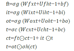
where the preliminary values are  = 0 and ℎ0 = 0 and the
operator ⊙ assumes the Hadamard product (element product). The
subscript t indexes the (next) time step.
= 0 and ℎ0 = 0 and the
operator ⊙ assumes the Hadamard product (element product). The
subscript t indexes the (next) time step.
•  input vector to the LSTM unit
•  forget gate’s activation vector
•  input/update gate’s activation vector
•  output gate’s activation vector
•  hidden state vector also known as output vector of
the LSTM unit
hidden state vector also known as output vector of
the LSTM unit
• t ∈ (-1,1)ℎ: cell input activation vector
•  cell state vector
•  weight matrices and bias
vector parameters which need to be learned during the training
period where the superscripts d and h refer to the number of input
features as well as the number of hidden units, correspondingly.
weight matrices and bias
vector parameters which need to be learned during the training
period where the superscripts d and h refer to the number of input
features as well as the number of hidden units, correspondingly.
Intrinsic activation functions
 sigmoid function.
 hyperbolic tangent function.
 hyperbolic tangent function, or
Reinforcement Learning Rule (Customized): Our seismic predictive analytics framework incorporates artificial neural networks, as shown above, that can work with rewards and penalties after each decision process, thus achieving a better and faster equilibrium. Our entirely ad hoc and game-theoretic-based reinforcement learning rule uses Q-learning mathematics. Modern reinforcement learning, a paradigm of Machine Learning (ML), is called Q-learning (Q=Quality). Most recently, an AI robot was taught to play a game using reinforcement learning.
Markov chains are mathematical models for predicting state transitions using probabilistic rules (e.g., 70% chance of coming to state A, initially commencing from the state E). A Markov Decision Process (MDP) is advantage extension of the Markov chain for modeling complex environments, allowing choices at each state and aggregating rewards for actions taken. This is the primary reason we refer to such instances as a stochastic, non-deterministic environment (randomized), e.g., for the same action performed in the same state, we may obtain various results (understand and do not comprehend (notifications)).
In our deployed reinforcement learning, that can be considered in the manner in which we model a game or antagonistic environment and our primary goal will be to maximize the reward we receive from that environment (Game-Theory). Our ultimate goal is to maximize the total reward as much as possible. However, trying to define the reward this way leads to two major issues:
• This sum can potentially diverge (go to infinity), which does not make sense since we want to converge it into maximization.
• We are considering as much for future rewards as we do for (inter)immediate rewards values.
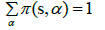
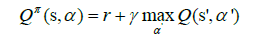
One way to correct these problems is to use a drop factor for future rewards. A policy is a utility function that informs what action to take while in a certain specialized state. This function is usually depicted as π(s,a) and has the probability of acting “a” in this state “s”. We want to retrieve the policy that maximizes the whole reward function. Moreover, as a probability distribution, the sum over all the possible actions must strictly be equal to 1.
Two well-defined “value functions” do exist. The state value
function, on the one hand and the action value function, on the other.
These functions are a good way to estimate the value, or how good
some state is, or how good ome action is, adjacently. The following
equation describes the former: 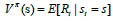 and the value of each
state is the expected total reward we can receive from that exact state.
It relies on the policy, which tells us how to make decisions. The
latter is shown with the following equation:
and the value of each
state is the expected total reward we can receive from that exact state.
It relies on the policy, which tells us how to make decisions. The
latter is shown with the following equation: 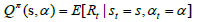 and the value of an action considered in some state is the expected
total reward we can receive, starting from that state and making that
action. It also relies on the exact policy.
and the value of an action considered in some state is the expected
total reward we can receive, starting from that state and making that
action. It also relies on the exact policy.
Now, we can represent the mathematical standards for our whole ANN environment. Observing the following diagram during the calculation can help us understand the (custom) reward-penalty process. This form of the Q-value is very abstract. It tackles stochastic environments, but we could translate it into a deterministic version. We finish in the same next state whenever we act and get the same reward. In that manner, we are not required to utilize a weighted sum with probabilities and the equation finally becomes the following.
Competitive learning: In this study’s scope, we underlined that competitive learning neural networks proved extremely accurate as clustering algorithmic candidates for earthquake prediction. Artificial neural networks use competitive learning and unsupervised learning in which nodes fight to respond to a portion of the input data. Competitive learning, a variation of Hebbian learning, functions by making every node in the network more specialized. It works effectively to locate clusters in the data. Models and methods such as vector quantization and self-organization (Kohonen maps) are based on competitive learning.
Neural networks with a hidden “competitive layer” layer are
typically used to implement competitive learning. Every competitive
neuron is described by a weight vector 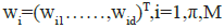 and
calculates the similarity measure between the input data xn =(xn,…
.,xnd)T nd the weight vector wi.
and
calculates the similarity measure between the input data xn =(xn,…
.,xnd)T nd the weight vector wi.
The competitive neurons “compete” with each other for each input vector, trying to determine the most comparable to that specific input vector. The winner neuron m sets its output om 1 and all other competitive neurons set their output oi=0, i=1,π, M, i ≠m.
Typically, the inverse of the Euclidean distance is used to calculate the similarity: ||x-wi|| between the input vector xn and the weight vector wi.
So, the question arises: How can an ad hoc deep learning technique, based on competitive learning, be developed to identify geolocation regions with seismic events? Neurons in a competitive layer learn to represent different regions of the input space where input vectors occur. P is a set of randomly generated but clustered test data points. Here, the data points are plotted.
A competitive network will be used to classify these points into natural classes. The following strategy will be to map our 2D input plane (6 × 10 matrix) to the output plane, which will be an 8-bit Boolean vector, with one TRUE-bit enabled each time. All rest bits will be FALSE, which corresponds to a new random direction (dis) placement (N, W, S, E, NW, NE, SW, SE) of the seismic event (re) occurrence upon the physical terrain. The neural network enabled to do so will be a competitive learning net with clustering. The network will be provided with the reinforcement learning capability from the output of the evaluation function f(●), which will reward or penalize the initial decisions of the random configuration. First, we simulate (create) the eight horizon directions with a (custom) Matlab code (Figure 3).

Figure 3: As clearly shown, we have eight clusters. The effort will be to map (train) each (6 ×10) matrix instance from the nn (e.g., nn=10000) Monte-Carlo instances into one only cluster. Note: (a) If re-enforcement learning is consistent, together with the DNN parameters, etc., 98% of the prediction time, the evaluation function should output a positive evaluation metric, for that prediction input; (b) As depicted from the image, classification has been successful. And the network has correctly classified the centroids of each cluster. The process demonstrates the competitive learning capabilities to cluster-classify the input.
Next, we set the number of epochs to train before stopping and training this competitive layer (which may take several seconds). We plotted the updated layer weights on the same graph.
Finally, let us predict a new prediction instance: That is, by creating a prediction input that is north-directed (e.g., with value ranges spaced around XY coordinates of the ‘N’ direction), the network will correctly classify the input in the fifth cluster, which is North, most of the time.
out=[00001000]
Game-theoretic learning approach
That way, we conclude with the Bellman equation in the context of Q-learning. The total value of an action a in some state s is the intermediate reward for taking that action, to which we sum the maximum expected reward we can receive in the next state. We define a custom equilibrium-based game in our ANN framework. The purpose of the game, the primary utility function in our Q-Learning model, is to use the reward as efficiently as possible to understand the appropriate action to perform. After each stage, the agent or player receives a 0-No guess submitted (only after reset), 1-Guess is lower than the target, 2-The guess equals the target, or 3 - The guess is greater than the target. The value(s) Guess is lower than the target, 2 - The guess equals the target, or 3-The guess is greater than the target. The value(s) ((min (action, self. number) + self bounds /(max(action, self number)+ self bounds))**2 are the predicted rewards. This is the squared proportion of how the agent estimated toward the objective.In an ideal world, a player can predict the taste of a higher reward and increase the pace at which his predictions are in that direction until the prize is reached; the reward reaches its maximum equilibrium. If an agent can learn the reward dynamics, it is possible to attain the maximum reward in two steps (one to detect the direction of the goal and the second to jump directly to the target based on the reward).
Sliding-Window learning approach
Our ad-hoc Sliding Window method is similar to the moving average computation procedure. A moving or rolling average is an estimate used in statistical analysis to evaluate data points by analyzing a sequence of averages, or means of flexible subsets of the entire data set. Additional dynamic aspects of our method include left-right feedback (in the window input/output), memory properties and sliding average properties. The “moving” window inputs the resource monitoring metrics and fully feeds back all of its complex outcomes in recursive cycles (Figure 4). It slides stochastically across the time axis (with an empirical static size of 8 value). Interestingly, the window travels sequentially (with a step size of 1) despite having an 8-size amidst the earlier axes. This behavior of our SW can be seen as an example of a low-pass filter used in signal processing and it can readily resemble a form of dynamic convolution.

Figure 4: The concept of sliding-window.
Prior research on convolutional sliding windows exists, but almost none has been applied to geophysics. The author(s) perform deep acceleration of the Gaussian filter using a short sliding window length by deploying Discrete Cosine Transform (DCT-1). In this paper, a fast constant-time Gaussian filter (O(1) GF) with low window length is shown. The constant time (O(1) in this filter indicates that the computational complexity per pixel is independent of the filter window length. The concept of O(1) GF based on the discrete cosine transform (DCT) forms the basis of the extensive design of the author(s) method. This framework uses a sliding transform to convolve each cosine term in O(1) per pixel, so it approximates a Gaussian kernel by a linear sum of cosine terms. If the window length is brief, DCT-1 comprises readily computed cosine values, namely 0, ± 1/2 and ± 1. Other types of DCT do not satisfy this behavior. Because of this, the author(s) has developed a method that uses DCT- 1 to accelerate the sliding transform while concentrating on short windows. Thus, an example proof-of-concept sliding transform of the DCT-3 method, with versatile use-case input features (either pixels or geological-oriented features), is given as
Results
Performance evaluation metrics
The networks we established above have only two possible outcomes: 0 indicates that an earthquake is not predicted to occur and 1 indicates that an earthquake is expected to occur. In general, we select the confusion matrix as one of the assessment criteria for such binary classifiers [81,82]. The actual meaning of each matrix element is listed in the earthquake prediction task.
• True Positives (TP): The quantity of times the model accurately forecasts the occurrence of an earthquake within the following experimental time frame.
• True Negatives (TN): The quantity of times the model accurately forecasts that there won’t be an earthquake during the following experimental time frame.
• False Positives (FP): The frequency with which the model incorrectly forecasts the occurrence of an earthquake within the following experimental time frame.
• False Negatives (FN): The quantity of times the model incorrectly forecasts that there won’t be an earthquake during the following experimental time frame.
Since an earthquake would result in an enormous loss if it is not foreseen to occur, we contend that FN presents the most serious issues. In the meantime, we will also keep the readers updated on FP. If the earthquake is anticipated, but does not occur, it can cause social problems during the evacuation drill. Thus, in our scenario, among the important evaluation metrics produced from the confusion matrix, the true positive rate linked to FN (TPR, also known as sensitivity or recall) and the positive predictive value connected to FP (PPV, also known as precision) are chosen. They have the following definitions.
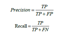
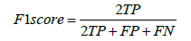
According to how the formulas are interpreted, precision is the proportion of actual earthquakes to anticipated ones. The term recall refers to the proportion of projected earthquakes to actual earthquakes. Every time there is an FN, the recall rate decreases. Similarly, each time an FP occurs, the accuracy rate suffers. Recall and precision are therefore expected to be as high as possible to minimize the penalty resulting from FN and FP. Another statistic, the f1 score, is used to counterbalance recall and precision’s effects on the evaluation. It is described as the precision and recall harmonic mean:
Lastly, presuming that the dataset is reasonably balanced, the test accuracy is included in the metrics to illustrate the model’s overall performance on unseen data clearly. It can be expressed as the proportion of accurate forecasts using the test data.
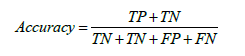
Clearly enough, we can tabulate the above machine learning model evaluation metrics (Table 1).
Lastly, we are particularly interested in the RMSE metric. The mean square error (MSE), mean absolute error (MAE) and root mean square error (RMSE) are computed to assess the model’s prediction accuracy for magnitude prediction. The prediction error is represented by MSE, the degree of variation between the expected and true values is reflected by RMSE and the average absolute error (AUE) between the predicted and observed values is represented by MAE. The following formula is used to determine the RMSE index:
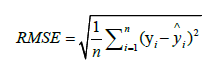
Where n is the number of predicted values, yi is the true value and is the predicted value.
Forecast results
Inside the full scope of the predictive dynamics potential capabilities of our artificial neural network framework, we performed a prior (before the real seismic event took place) and a posterior (afterward) on several occasions. We mainly focused on Greece’s geospatial territory and specific geodynamic areas with extensive seismic faults that can produce mega-earthquakes, like in 2021.
Predicting the next-day GR-law value: The first experimental data set, our objective was to forecast the next decimal value (with extremely low fractional relative tolerance to avoid loss of prediction accuracy) by using customized XGBoost (eXtreme Gradient Boosting) libraries along with solving a Game equilibrium to achieve maximum numerical efficiency for the next 24-hour mathematical value of the GR rule. Unlike gradient boosting, which operates as gradient descent in function space, XGBoost operates as Newton- Raphson; the connection to the Newton-Raphson method is made using a second-order Taylor approximation in the loss function. We efficiently implemented an ad hoc algorithm for generic unregularized XGBoost that acted as a (hyper)logistic regressor, or extrapolator. We targeted the geographical area of south Greece, specifically nearby Arkalochori, Crete (island), where on the 27 September, 2021 at 09:17 a.m. local time, a major seismic event of estimated magnitude MW 6.0. Figure 5 shows the major event and shows the progression of the time series of all earthquake phenomena from 27 September, 2021 to 07 October, 2021 as NOA, Greece, provided the data.

Figure 5: Major earthquake event (R 6.0) and aftershocks for Arkalochori, Crete, Greece on 27 September, 2021 to 07 October, 2021.
When entering the exact numerical data (interpolated and normalized) from the catalog of b values (NOA) in the database of the National Observatory of Athens into our custom library, we managed to extract the result of the next value of the GR law for the time step 2021.764, as shown and compared to Figure 6. It should be noted that the calculated RMSE value we received for the prediction data was 0.077438.

Figure 6: Machine-Learning (ML) prediction methods of the progressive b-value(s) for Arkalochori, Crete, Greece (year 2021) Note: (a) LinearRegression, (b) MLP Regressor, (c) XGBoost, (d) (HPC) XGBoost.
Predicting future GR-law values: This experimental section emphasized the gravity of future predictability of the progressive value b. As already mentioned in earlier sections, Earthquake Nowcasting (EN) evaluation is based on a new concept of time, termed natural time. Since counts of tiny events reflect a physical or natural time scale that characterizes the system’s behavior, event count models are also known as natural time models in physics. The basic premise is that enormous Earthquakes (EQ) will eventually occur to compensate for a lack of EQs in a local region enclosed within a broader seismically active zone. The theory states that over long periods and across wide spatial domains, the statistics of smaller regions will be equal to those of the larger region. Hence, small events can serve as a form of a “clock” to indicate the “natural time” that separates the big events [83].
This has been particularly the observed case for the Arkalochori, Crete, Greece (2021) seismic case study, according to the regions’ b-values. Thus, it remains important for seismologists to be able to forecast the future “trend” of the GR-law estimates both before and after major EQ events.
In this context, we applied four machine learning methodologies to project such potency from our ANN framework. The primary ML library (a) had been a standard linear regression model with weak exogeneity. This means that instead of being viewed as random variables, the predictor variables x might be treated as fixed values. This implies that predictor variables, for instance, are thought to be error-free or free of measurement errors. The second (b) ML library model was a Multilayer Perceptron Regressor with 2 thousand hidden layer-sized nodes and a 3-dimensional hidden layer network. The MLP regressor is trained iteratively because the parameters are updated at each time step by computing the partial derivatives of the loss function concerning the model parameters. The loss function may also include a regularization term that reduces the model’s parameters to avoid overfitting. Dense and sparse numpy arrays of floating point values are the data types this implementation uses. The (c) ML model deployed had been a conventional XGBoost library, whereas in (d), we decided to invoke a High-Performance Computing (HPC), or the most efficient deep learning network of separate XGBoost libraries both wise optimized in terms of precision, recall and accuracy.
Our general (future) adjustment accuracy depends mainly on
the efficacy of strengthening the gradient tree (extreme) [84]. It is
not possible to optimize the tree ensemble model in the regularized
learning objective of the conventional tree boosting in Euclidean space
using conventional optimization techniques since it has functions as
parameters. Rather, the model undergoes additive training. Formally,
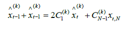
we will need to add feet to minimize the following objective: let  be the forecast of the i-th occurrence in the t-th iteration.
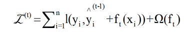
This indicates that, by the regularized learning objective of the conventional tree boosting, we add the foot greedily if it most improves our model. The objective can be easily optimized in the generic setting using a second-order approximation. The previous equation can be applied as a classification function to assess the quality of a tree structure q. This score is produced for a wider variety of objective functions than the impurity score used to evaluate decision trees. Generally speaking, it is impossible to list all potential tree structures q. Instead, a greedy algorithm is employed, which begins with a single leaf and iteratively builds branches to the tree. We observe the four ML models in Figure 8. From all the benchmarks above, (d) HPC-XGBoost has the highest accuracy because it works like a segmented network of connected optimized (c) individual XGB libraries. In contrast, the least accurate ML methodology belongs to the MLP regressor (b), probably due to minor overfitting issues.
Next-day seismic prediction for Arkalochori, Crete, Greece: In the second set of experimental trials, we applied the competitive learning features of our now casting seismic architecture embedded with the LSTM potentials and the sliding window technique we described before. Again, we selected the same geographical area of Greece (Arkalochori, Crete) during a calmer earthquake activity period (arbitrary selection). We aimed to predict the set of four-tuple characteristics ((a) latitude, (b) longitude, (c) focal depth and (d) magnitude) of the potential seismic activities of the next 24 hours. Figure 7 projects the forecasted and real events that occurred with respect to the seismic centroids. The level of earthquake now-casting accuracy in this scenario seems compelling.
However, even after the main EQ event time slot, we followed the exact concept of Natural Time methodology, according to, to project the predictability of our software framework for aftershocks. There were two technical reasons for this approach. First, the seismicity order parameter, k_1: Its minimum indicates when Seismic Electric Signal (SES) activities begin and its value (=0.070) indicates when the system reaches the critical stage. There is an aftershock k_1 interval period, which we approximated in this trial here. The second is the change in entropy, or ΔS, under time reversal: Its value, when minimized a few months ahead of time, indicates the beginning of precursory phenomena; its fluctuations, when the ΔS minimum appears, show a clear increase, indicating the beginning of the preparation of EQ, as explained by the physical model that served as the inspiration for the SES research.
These two quantities were intrinsically utilized to study precursory, particularly the metacursory phenomena following the major EQs in Arkalochori (year 2021). One of the main withholding concepts of our ANN framework is the “topological” and “chronological” locality of reference, as derived from the previous meta-information parameters of the natural time technique (k_1 and ΔS). Specifically, despite the high but not maximum-arising entropy levels of the NTEQ prediction, the stochasticity of the phenomena leaves us with the opportunity to predict, via the holistic artificial neural network strategy, location/time occurrences that happened recently with the ML possibility to occur again in the nowcasted future (Geo/Timelocality of reference property) (Figure 7).

Figure 7: Machine Learning Earthquake Prediction (USGS) for Arkalochori, Crete 16 July, 2022.
Long-term seismic prediction
Theva, Voitiea, Central Greece: Perhaps the most important and life-critical applicability scenario for citizens of a highly accurate seismic forecasting mechanism is to be able to make agile seismic predictions for major events in any geographical territory as early as possible before the phenomena take place. On 28 December, 2022 at 12:24:21 local Greece time, a moderate earthquake shock occurred near Theva, in Voitiea district, Greece, measured at MW=4.9, then by the NOA instruments. Even from the date back to the 24 October, 2022 our Artificial Neural Network framework successfully predicted the exact 4-tuple seismic feature set with extreme accuracy, as shown below, both graphically and numerically (Figure 8 and Table 2).

Figure 8: Machine Learning Earthquake Prediction,  ≥ 3.0, (USGS) for Thiva, Boeotia, Central Greece [25 October, 2022 ≤ 31
December,2022] Note: (a) Real; (b) Forecasted major shock [28 December, 2022 12:24:21 (GMT)], Theva, Voitiea, Greece.
≥ 3.0, (USGS) for Thiva, Boeotia, Central Greece [25 October, 2022 ≤ 31
December,2022] Note: (a) Real; (b) Forecasted major shock [28 December, 2022 12:24:21 (GMT)], Theva, Voitiea, Greece.
| Lat (°N) | Long (°E) | Focal Depth (km) | Magnitude (R) | |
|---|---|---|---|---|
| Predicted data* | 38.5267 | 23.6367 | 8 | 5.1 |
| Real data | 38.5652 | 23.6906 | 13 | 4.9 |
| *Date of exact Machine-learning seismic prediction: 24 October, 2022 | ||||
Table 2: Numerical comparison matrix of the seismic forecasting accuracy of the [28 December,2022 12:24:21 (GMT)] event, Theva, Voitiea, Greece.
Sitia, Crete, South Greece: The seismic year 2021 in Greece was particularly active, with three main EQs occurring in different (sub)regions with different geophysical traits and seismic fault indications. The MW=6.4 in the Sitia Crete EQ on 12 October, 2021 was one of those. In this particular use case, we “backtested” our ANN software with historical datasets 15 years before this exact EQ occurred in the same nearby geographical region as input datasets. We project and analyze the deep learning results of competitive learning (+sliding window / NTA) in Figure 8. Again, the numerical accuracy of the magnitude scale, time prediction interval and especially the longitude/latitude precision seems quite emphatic.
Natural-time analysis (NTA), examined in earlier sections, is useful for determining whether a complex system has reached a critical stage and for revealing the system’s dynamical evolution. Because of this, NTA can be extremely helpful in anticipating future catastrophic catastrophes, such as the advent of huge EQs. In this research effort, we demonstrate that if NTA analysis is codeployed with advanced machine learning and game-theoretic mathematical techniques, it can project real practicality not only to now casting but also to forecasting efforts for applied predictive seismology.
Tyrnavos, North Greece: Our next studied seismic use case, one of the major EQ events that shocked central Greece in 2021, was in Tyrnavos. The main event occurred with MW=6.3 in Tyrnavos on 3 March, 2021. Again, we performed a validation analysis of the backtest of our predictive software and depicted the real and predicted comparison results in Figure 9.

Figure 9: Machine Learning Earthquake Prediction, ≥ 4.0, (USGS) for Sitia, Crete, Greece [complete year 2021] Note: (a) Real; (b)
Predicted major shock (R 6.4), Sitia, Crete, Greece (2021).
The same as before, the overall 4-tuple ((a) latitude, (b) longitude, (c) focal depth and (d) magnitude) numerical accuracy, or match, between what “would” happen and what “really” happened is quite interesting. Besides the forecasting accuracy of the main shock, the predictability capabilities of the aftershocks that took place from our ANN software architecture are also worth noticing.
Here, we also used (as a proof of comparison) the most recent
version of Megacities Earthquake Nowcasting software [85,86].
Based on the NTA equations in the Introduction section and the
assumption that  in each catalog case, we calculated the EPS
using the empirical CDF computed in the large region. We also
considered the epicenter of each of the strong EQs in 2021 as the
center of the circular zone. To estimate the EPS for EQs of magnitude
greater than or equal to
in each catalog case, we calculated the EPS
using the empirical CDF computed in the large region. We also
considered the epicenter of each of the strong EQs in 2021 as the
center of the circular zone. To estimate the EPS for EQs of magnitude
greater than or equal to  =6.5, Rundle et al. [39], [83] estimated
 =400 km and
  =200 km around the Greek capital, Athens (Figure
1).
=200 km around the Greek capital, Athens (Figure
1).
Comprehensive forecast analysis for whole Greece territory -
year 2021: In this Section, we holistically deployed and mapped our
seismic nowcasting software to foresee if we could “pick” the 3 major
EQs events that shocked Greece in the quite active year of 2021 ((1)
(EQ Name) Tyrnavos (EQ Date) 3 March, 2021 (Lat) 39.8 (Long)
22.2 (MW) 6.3 (EPS) 98.5, (2) (EQ Name) Arkalohorion Crete (EQ Date) 27 September, 2021 (Lat) 35.2 (Long) 25.3 6.0 (EPS) 62.0
and (3) (EQ Name) Sitia Crete (EQ Date) 12 October, 2021 (Lat) 35.2
(Long) 26.2 6.4 (EPS) 34.3). Our competitive learning neural
networks made it feasible to forecast both EQ occurrences for the
same year (2021) timeframe. Alongside, more moderate to minor
magnitude scaled events were predicted across the Greek territory,
with some non-avoidable FP/FN instances appearing alike in the
same right-most sub-plot figure. What we can conclude from this trial
case is that both atomically (as shown in the case studies before) and
comprehensively, the predictive software ANN (NTA-based) can spot
moderate
6.0 (EPS) 62.0
and (3) (EQ Name) Sitia Crete (EQ Date) 12 October, 2021 (Lat) 35.2
(Long) 26.2 6.4 (EPS) 34.3). Our competitive learning neural
networks made it feasible to forecast both EQ occurrences for the
same year (2021) timeframe. Alongside, more moderate to minor
magnitude scaled events were predicted across the Greek territory,
with some non-avoidable FP/FN instances appearing alike in the
same right-most sub-plot figure. What we can conclude from this trial
case is that both atomically (as shown in the case studies before) and
comprehensively, the predictive software ANN (NTA-based) can spot
moderate  and mega-earthquake events with considerable
(4-tuple) accuracy (Figures 10 and 11).
and mega-earthquake events with considerable
(4-tuple) accuracy (Figures 10 and 11).

Figure 10: Machine Learning Earthquake Prediction, ≥ 4.5, (USGS) for Tyrnavos, Greece [complete year 2021] Note: (a) Real ;(b)
Predicted major shock (R 6.3), Tyrnavos, Greece (2021).

Figure 11: Machine Learning Earthquake Prediction (USGS) for Greece [complete year 2021] Note: (a) Real; (b) Predicted major and minorshock event(s), Greece (2021).
Error validation analysis: Based on what we discussed and assumed in Section 5.1, we depict in Figure 11 the 2-dimensional confusion matrix of our holistic framework for clustering in seismic nowcasting. Hereby, we attach the True Positive(s) and other accuracy estimation metrics. We can safely claim that our machine learning methodology (co-deployed with the sliding-window technique) can reach even a (beyond) 6-month long-term earthquake forecasting accuracy of at least 90%. By continuing to work and improving our models and their hyper parameters, we are optimistic that that we can obtain even higher precision-recall accuracy (Figure 12).

Figure 12: Confusion error matrix of our framework.
Discussion
The scientific luxury of obtaining a network of seismographic instruments and next-generation Internet of Things microseismic sensors that can aggregate in real time a massive amount of earthquake data from beneath the earth’s surface would be an additional feature for any research attempts like the one above that aims to leverage state of the art Artificial Intelligence (AI) to predict shock events in the short and long term. At first glance, we can increase the number of layers in each network to enable each network to learn more consecutive properties from the data. Then, improving the hyperparameters is another choice.
As Future Work for our research project, we will deploy explicit next-generation (hybrid) transformer networks, focusing on exploiting eXplainable AI (XAI) techniques and building Large Language Models (LLMs). The latter are known to possess extreme potency in language detection and language generation. The research field of predicting earthquakes via generative AI (GPT-4) would be quite interesting to construct and experiment on.
Ultimately, the investigation showed that earthquake prediction remains a difficult issue. Various deep learning techniques can be applied separately or in combination to determine the best approach for these time series forecasting problems.
Conclusion
this work, we investigated the feasibility of applying various fully ad-hoc machine learning techniques and an LSTM/Competitive learning deep neural network to forecast the maximum magnitudes and frequency of earthquakes in the Greek area. As input features, we computed and retrieved seismicity metrics associated with earthquake occurrence from the catalog. The results demonstrated that the research potential has been quite promising in categorizing significant earthquakes.
The results provide evidence in favor of the theory that small earthquakes can provide useful information for forecasting larger earthquakes in the future and present a viable method for doing so. Furthermore, the results offer valuable information on which elements consistent with physical interpretation are critical for earthquake prediction.
Although this study has much room for improvement and scientific speculation, it offers a possible route to increase the accuracy of earthquake prediction in the future.
References
- Vardaan K, Bhandarkar T, Satish N, Sridhar S, Sivakumar R, et al. (2019) Earthquake trend prediction using long short-term memory RNN. Int J Electr Com Eng 9(2):1304-1312.
- Wang Q, Guo Y, Yu L, Li P (2017) Earthquake prediction based on spatio-temporal data mining: An LSTM network approach. IEEE Trans Comput 8(1):148-158.
- Boucouvalas AC, Gkasios M, Tselikas NT, Drakatos G (2015) Modified-fibonacci-dual-lucas method for earthquake prediction. SPIE proceed 9535:400-410.
- Chouliaras G (2009) Seismicity anomalies prior to 8 June 2008, M w=6.4 earthquake in Western Greece. Nat Haz and Ear Syst Sci 9(2):327-335.
- Fan J, Chen Z, Yan L, Gong J, Wang D (2015) Research on earthquake prediction from infrared cloud images. SPIE 9815:87-92.
- Hayakawa M, Yamauchi H, Ohtani N, Ohta M, Tosa S, et al. (2016) On the precursory abnormal animal behavior and electromagnetic effects for the Kobe earthquake (M~6) on April 12, 2013. J Earthq Res 5(03):165.
- Moustra M, Avraamides M, Christodoulou C (2011) Artificial neural networks for earthquake prediction using time series magnitude data or seismic electric signals. Expert Syst App 38(12):15032-15039.
- Yousefzadeh M, Hosseini SA, Farnaghi M (2021) Spatiotemporally explicit earthquake prediction using deep neural network. Soil Dyn Earthq Eng 144:106663.
- Ruiz L, Gama F, Ribeiro A (2019) Gated graph convolutional recurrent neural networks. EUSIPCO 1-5.
- Kavianpour P, Kavianpour M, Jahani E, Ramezani A (2023) CNN-BiLSTM model with attention mechanism for earthquake prediction. J Sup comput 79(17):19194-19226.
- Du X (2022) Short-term earthquake prediction via recurrent neural network models: Comparison among vanilla RNN, LSTM and Bi-LSTM.
- Panakkat A, Adeli H (2007) Neural network models for earthquake magnitude prediction using multiple seismicity indicators. Int J Neural Syst 17(1):13-33.
- Asencio-Cortés G, Martínez-Álvarez F, Morales-Esteban A, Reyes J (2016) A sensitivity study of seismicity indicators in supervised learning to improve earthquake prediction. Know Based Syst 101:15-30.
- Asim KM, Idris A, Iqbal T, Martínez-Álvarez F (2018) Seismic indicators based earthquake predictor system using genetic programming and adaboost classification. Soil Dyn Earthq Eng 111:1-7.
- Martínez-Álvarez F, Reyes J, Morales-Esteban A, Rubio-Escudero C (2013) Determining the best set of seismicity indicators to predict earthquakes. Two case studies: Chile and the Iberian Peninsula. Know Bas Syst 50:198-210.
- Florido E, Asencio–Cortés G, Aznarte JL, Rubio-Escudero C, Martínez–Álvarez F (2018) A novel tree-based algorithm to discover seismic patterns in earthquake catalogs. Comput Geosci. 115:96-104.
- Rundle JB, Donnellan A, Fox G, Crutchfield JP (2022) Nowcasting earthquakes by visualizing the earthquake cycle with machine learning: A comparison of two methods. Sur Geophy 43(2):483-501.
- Wang X, Zhong Z, Yao Y, Li Z, Zhou S, et al. (2023) small earthquakes can help predict large earthquakes: A machine learning perspective. App Sci 13(11):6424.
- Chouliaras G (2009) Investigating the earthquake catalog of the national observatory of Athens. Nat Haz Ear Syst Sci 9(3):905-912.
- Mignan A, Chouliaras G (2014) Fifty years of seismic network performance in Greece (1964–2013): Spatiotemporal evolution of the completeness magnitude. Seis Res Let 85(3):657-667.
- National observatory of Athens, Institute of Geodynamics. Recent Earthquakes.
- Rundle JB, Turcotte DL, Donnellan A, Grant LL, Luginbuhl M, et al. (2016) Nowcasting earthquakes. Earth Spac Sci 3(11):480-486.
- Varotsos PA (2001) Spatio-temporal complexity aspects on the interrelation between seismic electric signals and seismicity. Pract Athens Acad 76:294.
- Varotsos PA, Sarlis NV, Skordas ES (2002) Long-range correlations in the electric signals that precede rupture. Phys Rev 66(1):011902.
- Varotsos P, Sarlis N, Skordas E (2002) Seismic Electric Signals and Seismicity: On a tentative interrelation between their spectral content. Acta Geophys 50(3):337-354.
- Varotsos PA, Sarlis NV, Tanaka HK, Skordas ES (2005) Similarity of fluctuations in correlated systems: The case of seismicity. Phys Rev E 4:041103.
[Crossref] [Google Scholar][Pubmed]
- Varotsos P, Sarlis NV, Skordas ES (2011) Natural time analysis: The new view of time: Precursory seismic electric signals, earthquakes and other complex time series. Spri Sci Busin Med.
- Pasari S. Nowcasting earthquakes in the Bay of Bengal region (2019) Pure Appl Geophy 176:1417-32.
- Pasari S, Verma H, Sharma Y, Choudhary N (2023) Spatial distribution of seismic cycle progression in northeast India and Bangladesh regions inferred from natural time analysis. Acta Geophysica 71(1):89-100.
- Tokuji UT (1984) Estimation of parameters for recurrence models of earthquakes. Bul Earthquake Res Inst Univ Tokyo. 59:53-66.
- Pasari S, Dikshit O (2015) Distribution of earthquake interevent times in northeast India and adjoining regions. Pure Appl. Geophys. 172:2533-44.
- Pasari S, Dikshit O (2015) Earthquake interevent time distribution in Kachchh, Northwestern India. Earth Planets Space 67:1-7.
- Rundle JB, Luginbuhl M, Giguere A, Turcotte DL (2018) Natural time, nowcasting and the physics of earthquakes: Estimation of seismic risk to global megacities. Pure Appl. Geophys 175:123-36.
- Luginbuhl M, Rundle JB, Hawkins A, Turcotte DL (2018) Nowcasting earthquakes: A comparison of induced earthquakes in Oklahoma and at the Geysers, California. Pure Appl. Geophys 175:49-65.
- Luginbuhl M, Rundle JB, Turcotte DL (2019) Natural time and nowcasting earthquakes: Are large global earthquakes temporally clustered?. Earth Multi Hazards Around Pacific Rim 2019:137-46.
- Rundle JB, Donnellan A (2020) Nowcasting earthquakes in Southern California with machine learning: Bursts, swarms and aftershocks may be related to levels of regional tectonic stress. Earth Space Science7(9):e2020EA001097.
- Rundle JB, Stein S, Donnellan A, Turcotte DL, Klein W, et al. (2021) The complex dynamics of earthquake fault systems: New approaches to forecasting and nowcasting of earthquakes. Rep Prog Phy 84(7):076801.
- Rundle JB, Donnellan A, Fox G, Crutchfield JP (2022) Nowcasting earthquakes by visualizing the earthquake cycle with machine learning: A comparison of two methods. Surv Geophysics 43(2):483-501.
- Rundle JB, Donnellan A, Fox G, Crutchfield JP, Granat R (2021) Nowcasting earthquakes: Imaging the earthquake cycle in California with machine learning. Earth Space Sci 12 :e2021EA001757.
- Rundle JB, Donnellan A, Fox G, Ludwig LG, Crutchfield J (2023) Does the Catalog of California Earthquakes, With Aftershocks Included, Contain Information About Future Large Earthquakes?. Earth Space 10(2):e2022EA002521.
- Perez OJ, Angulo BF, Sarlis NV (2020) Nowcasting avalanches as earthquakes and the predictability of strong avalanches in the Olami-Feder-Christensen model. Entropy 28;22(11):1228.
[Crossref] [Google Scholar][Pubmed]
- Varotsos P, Sarlis N, Skordas E (2020) Natural Time Analysis: The New View of Time, Part II: Advances in Disaster Prediction Using Complex Systems. Springer Nature.
- Varotsos PA, Sarlis NV, Skordas ES, Lazaridou MS (2008) Fluctuations, under time reversal, of the natural time and the entropy distinguish similar looking electric signals of different dynamics. J Appl Phys 103(1).
- Sarlis NV, Skordas ES, Lazaridou MS, Varotsos PA (2008) Investigation of seismicity after the initiation of a Seismic Electric Signal activity until the main shock. Proc Jpn Acad Ser B Phys Biol Sci 84(8):331-43.
[Crossref] [Google Scholar][Pubmed]
- Uyeda S, Kamogawa M (2008) The prediction of two large earthquakes in Greece. Eos Trans 89: 363.
- Uyeda S, Kamogawa M (2010) Comment on “The prediction of two large earthquakes in Greece”. Eos Trans 91(18):162.
- Uyeda S, Kamogawa M, Tanaka H (2009) Analysis of electrical activity and seismicity in the natural time domain for the volcanic‐seismic swarm activity in 2000 in the Izu Island region, Japan. J. Geophys. Res 114(B2).
- Sarlis NV, Skordas ES, Varotsos PA, Nagao T, Kamogawa M, et al. (2013) Minimum of the order parameter fluctuations of seismicity before major earthquakes in Japan. Proc Natl Acad Sci 110(34):13734-8.
- Sarlis NV, Skordas ES, Varotsos PA, Nagao T, Kamogawa M, et al. (2015) Spatiotemporal variations of seismicity before major earthquakes in the Japanese area and their relation with the epicentral locations. Proc Natl Acad Sci 112(4):986-9.
- Varotsos PA, Sarlis NV, Skordas ES, Uyeda S, Kamogawa M (2010) Natural-time analysis of critical phenomena: The case of seismicity. Europhys Lett 92(2):29002.
- Skordas ES, Christopoulos SR, Sarlis NV (2020) Detrended fluctuation analysis of seismicity and order parameter fluctuations before the M7. 1 Ridgecrest earthquake. Natural Hazards 100:697-711.
- Sarlis NV, Skordas ES, Varotsos PA, Ramírez RA, Flores MEL (2018) Natural time analysis: On the deadly Mexico M8. 2 earthquake on 7 September,2017. Physica A: Statis Mech App 506:625-34.
- Sarlis NV, Skordas ES, Varotsos PA, Ramírez RA, Flores MEL (2019) Identifying the occurrence time of the deadly Mexico M8. 2 earthquake on 7 September,2017. Entropy 21(3):301.
- Perez OJ, Varotsos PK, Skordas ES, Sarlis NV (2021) Estimating the epicenter of a future strong earthquake in Southern California, Mexico and Central America by means of natural time analysis and earthquake nowcasting. Entropy 23(12):1658.
- Mintzelas A, Sarlis NV (2019) Minima of the fluctuations of the order parameter of seismicity and earthquake networks based on similar activity patterns. Physica A: Statis Mech App 527:121293.
- Varotsos PK, Perez-Oregon J, Skordas ES, Sarlis NV (2021) Estimating the epicenter of an impending strong earthquake by combining the seismicity order parameter variability analysis with earthquake networks and nowcasting: Application in the Eastern Mediterranean. Appl Sci 11(21):10093.
- Sarlis NV, Christopoulos SR, Skordas E (2015) Minima of the fluctuations of the order parameter of global seismicity. Chaos 25(6).
- Sarlis NV, Skordas ES, Mintzelas A, Papadopoulou KA (2018) Micro-scale, mid-scale and macro-scale in global seismicity identified by empirical mode decomposition and their multifractal characteristics. Sci Rep 8(1):9206.
- Christopoulos SR, Varotsos PK, Perez OJ, Papadopoulou KA, Skordas ES, et al. (2022) Natural time analysis of global seismicity. Applied Sciences 12(15):7496.
- Varotsos PA, Sarlis NV, Skordas ES (2003) Attempt to distinguish electric signals of a dichotomous nature. Phy Rev E 68(3):031106.
- Varotsos PA, Sarlis NV, Skordas ES, Lazaridou MS (2004) Entropy in the natural time domain. Phy Rev E 70(1):011106.
- Varotsos PA, Sarlis NV, Tanaka HK, Skordas ES (2005) Some properties of the entropy in the natural time. Phy Rev E 71(3):032102.
- Lesche B(1982) Instabilities of Rényi entropies. J Stat phys 27(2):419-22.
- Lesche B (2004) Renyi entropies and observables. Phys Rev E 70: 017102.
- Sarlis NV (2017) Entropy in natural time and the associated complexity measures. Entropy 19:177.
- Sarlis NV, Skordas ES, Varotsos PA (2018) A remarkable change of the entropy of seismicity in natural time under time reversal before the super-giant M9 Tohoku earthquake on 11 March,2011. Europhys Lett 124(2):29001.
- Varotsos PA, Sarlis NV, Skordas ES (2018) Tsallis entropy index q and the complexity measure of seismicity in natural time under time reversal before the M9 Tohoku earthquake in 2011. Entropy 20(10):757.
- Skordas ES, Sarlis NV, Varotsos PA (2020) Identifying the occurrence time of an impending major earthquake by means of the fluctuations of the entropy change under time reversal. Europhys Lett 128(4):49001.
- Varotsos PA, Sarlis NV, Skordas ES (2020) Self-organized criticality and earthquake predictability: A long-standing question in the light of natural time analysis. Europhys Lett (2):29001.
- Ramírez RA, Flores MEL, Sarlis NV, Varotsos PA ()2018 The complexity measures associated with the fluctuations of the entropy in natural time before the deadly México M8. 2 earthquake on 7 September,2017. Entropy 20(6):477.
- Flores MEL, Ramírez RA, Perez OJ, Sarlis NV, Skordas ES, et al. (2020) Natural time analysis of seismicity within the mexican flat slab before the M7. 1 earthquake on 19 September,2017. Entropy. 2(7):730.
- Varotsos PA, Sarlis NV, Skordas ES (2022 ) Order parameter and entropy of seismicity in natural time before major earthquakes:Recent results. Geosciences 12(6):225.
- Varotsos P, Alexopoulos K (1984) Physical properties of the variations of the electric field of the earth preceding earthquakes I. Tectonophysics 110(1-2):73-98.
- Varotsos P, Alexopoulos K, Nomicos K, Lazaridou M (1986) Earthquake prediction and electric signals. Nature 322(6075):120.
- Varotsos P, Lazaridou M (1991) Latest aspects of earthquake prediction in Greece based on seismic electric signals. Tectonophysics 188(3-4):321-47.
- Varotsos P, Alexopoulos K, Lazaridou M (1993) Latest aspects of earthquake prediction in Greece based on seismic electric signals, II. Tectonophysics 224(1-3):1-37.
- Varotsos PA (2005) The physics of seismic electric signals. Terrapub 338.
- Varotsos PA, Sarlis NV, Skordas ES (2019) Phenomena preceding major earthquakes interconnected through a physical model. Ann Geophys. 37:315–324.
- Varotsos PA, Sarlis NV, Skordas ES, Lazaridou MS (2013) Seismic Electric Signals: An additional fact showing their physical interconnection with seismicity. Tectonophysics 589:116-25.
- Chouliaras G (2009) Seismicity anomalies prior to 8 June, 2008, M w=6.4 earthquake in Western Greece. Nat Hazards Earth Syst Sci 9(2):327-35.
- Shaikh SA (2011) Measures derived from a 2×2 table for an accuracy of a diagnostic test. J Biom Biostat 128:1-4.
- Kim J, Yang I (2020) Hamilton-Jacobi-Bellman equations for Q-learning in continuous time. Learn Dyn Cont 739:748.
- Chouliaras G, Skordas ES, Sarlis NV (2023) Earthquake nowcasting: Retrospective testing in Greece. Entropy. 25(2):379.
- Chen T,Guestrin C (2016). XGBoost: A Scalable Tree Boosting System. Int Conf Knowled Dis Data Mining.
- Yano T, Sugimoto K, Kuroki Y, Kamata SI (2018) Acceleration of Gaussian filter with short window length using DCT-1. IEEE.129-132.
- Rundle J (2023) Megacities Earthquake Nowcasting. Zenodo.
[Crossref]