Review Article, Res Rep Math Vol: 2 Issue: 2

Mathematical Perspectives in Plasma Turbulence

Cheverry C^*

Institut Mathematique de Rennes, Campus de Beaulieu, France

*Corresponding Author : Christophe Cheverry
Institut Mathematique de Rennes, Campus de Beaulieu, 263 avenue du General Leclerc, CS 74205, 35042 Rennes, France
E-mail: christophe.cheverry@univ-rennes1.fr

Received: January 04, 2018 Accepted: January 05, 2018 Published: April 12, 2018

Citation: Cheverry C (2018) Mathematical Perspectives in Plasma Turbulence. Res Rep Math 2:2

Abstract

Keywords: Plasma turbulence; Coherent structures; Intermittency; Waveparticle interaction; Resonance; Nonlinear geometric optics; Dynamical systems

Introduction

A largely unsolved theoretical issue, in connection with the modeling of stars, magnetospheres and fusion devices, is the consistent kinetic treatment of phenomena occurring in collisionless magnetized plasmas. A related challenge, with practical applications, is to determine whether and how ionized gases can be confined long enough by a magnetic field?

For simplicity, we consider here that the plasma is contained in an open spatial domain and that it is made of electrons in a background of stationary protons. These electrons are described by a distribution function f (t, x,ξ) which gives at the time their probability density on the phase space Furthermore, they are subjected to the influence of a strong exterior inhomogeneous magnetic field ε-1 Be(x). The function Be(.)is prescribed. It is assumed to be smooth, nowhere zero and of size one. The dimensionless number ε is small:

(1)

The parameter ε is the inverse of the electron gyrofrequency. The electrons are also impacted by a self-consistent electromagnetic field, denoted by t(E,B) (t, x).

The confined plasmas contain a whole spectrum of collective oscillations known as plasma waves. They are not quiescent at all. That is probably why they are not fully understood. The first difficulty arises from the complex microscopic phase-space dynamics of charged particles. In strongly magnetized plasmas, these dynamics are mainly determined by the large term “ε-1 Be(.). Pertinent issues are therefore about coherent turbulent structures. This amounts to describing the content of f (.), as it can be governed by the sole action of “ε-1 Be(.). Such aspects will be examined in Section 2.

In practice, the charged particles also feel the interplay of the distribution function f (.) with the self-consistent electromagnetic field (E,B)(.), and therefore other difficulties are issued from waveparticle interactions [1-34]. This consists in the understanding of the coupling between f, E and B. Such aspects will be investigated in Section 3.

Then, Section 4 informs the reader about ongoing developments in the subject, which related to nonlinear mechanisms.

This text is also an occasion to clarify (in the context of collisionless magnetized plasmas) different notions of turbulence (labelled by i, ii, iii and iv) as well as various concepts of resonance (labelled by a, b and c).

Let us now formulate the above problems in mathematical terms. The preceding questions can be addressed within the framework of the Relativistic Vlasov-Maxwell description, the RVM system in abbreviated form. This system is composed by the Vlasov equation:

∂tf +[υ(ξ) . ∇x] f- ε−1 [υ(ξ)∧Be(x)]. ∇f = [E+υ(ξ)∧B]. ∇f (2)

together with the Maxwell’s equations:

∂tE − ∇x × B = �?·(f ) , div E = ρi − ρ(f ), (3)

∂tB + ∇x × E = 0 , div B = 0 . (4)

In (2), the vector υ(ξ) is the normalized velocity, whereas the scalar is the Lorentz factor:

(5)

In (3), the (positive) constant ρi represent some (given) density of charge issued from ions. The two expressions �?· (f)(t, x) and ρ(f)(t, x) stand respectively for the electric current and the electronic density of charge. They can be computed from f (.) according to :

(6)

The RVM system (2)-(6) on (f;E;B) (.) is clearly self-contained. Since all equations are known, a complete study is in principle possible. However, the discussion is highly complicated by the presence of the parameter ε. As already mentioned, the smallness of ε«1 is physically very relevant. Since ε appears at the level of (2), all functions f, E and B depend on ε∈[0,1]. The same applies to the fields X and Ξ, that will be subsequently introduced, see (7) and (8). However, for the sake of simplicity, the link to ε∈]0,1] will not be marked at the level of f , E, B, X, Ξ, X and Ξ.

The study of (2)-(6) has long been addressed in theoretical physics and mathematics. Due to the importance of the smallness assumption ε ∈1, it has been investigated through the development of asymptotic analysis, when ε goes to 0. The aim of this text is to present recent results on this topic (Sections 2 and 3) and works in progress (Section 4).

Charged Particle Dynamics and Coherent Structures

This section is devoted to the study of (2) in the absence of a selfconsistent electromagnetic field, that is when E ≡ 0 and B ≡ Σ0. Then, the Σ charged particles (here electrons) only respond to the external Lorentz force ε−1 [υ(ξ) ∧Be(x)], which appears as the most singular term of (2). In this simplified framework, we are just faced with the dynamical system:

(7)

The electrons follow the characteristics of the Vlasov equation, which are the integral curves associated to the ordinary differential equation (7). The magnetic field is uniform when:

Then, the charged particles move along helical paths [20]. But in the presence of a prescribed inhomogeneous magnetic field, they can move along much more complex trajectories. The complexity arises from the variations of the function Be(.). Typically, there are three basic periodic motions: gyration, bounce, and drift. These three basic motions imply three different frequencies appearing during three successive intervals of times: t∼ ε (gyration), t∼1 (bounce) and t∼ ε-1 (drift). Note that the ions undergo similar behaviors but on much longer time scales (multiply t by the proton-to-electron mass ratio ×103). Define τ:= εt. In what follows, times τ such that τ∼1 (or equivalently t∼ ε−1) will be referred as long times. The description of these motions has long been studied through the hamiltonian formalism, through canonical transformations to action and angle variables [2-38]. This is still a highly topical issue, see for instance [21,22] (Figure 1).

Using τ in place of t, defining (X, Ξ ) (τ ) := (X, Ξ)(ε−1 τ ), the system (7) is replaced by:

(8)

In comparison with the lessons learned from KAM theory [2] and gyrokinetics [21], an innovative aspect of [6,7] is a better Eulerian specification of the flow field, which is viewed at fixed scales and with a long-term perspective. As a matter of fact, the length and time scales are adjusted in view of concrete applications. The first article [6] deals with the Earth’s magnetosphere, with an external magnetic field Be(·) given by the dipole model of the geomagnetic field; the second contribution [7] considers the case of tokamaks, with Be(.) isuued from general magnetic flux surfaces. The system (7) is almost integrable, but what remains at fixed scales, modulo a hierarchy in powers of ε, is just inerrability or oscillations. To illustrate this assertion, we recall below the main statement of [7].

Theorem [global and long time dynamics of charged particles in axisymmetric devices] The phase space can be decomposed into a finite number of disjoint open subsets such that:

Fix any j∈{0,…, m} and any compact subset Uniformly in (x, ξ) ∈ K, we can find some ε0 ∈ ]0, 1[, a time , two phases:

ε ∈ ]0, ε0], and a sequence of profiles:

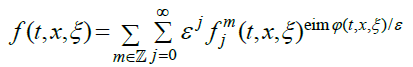
such that the asymptotic behavior when ε ∈ ]0, ε0[ goes to zero of the solution t(X, Ξ )(τ, x, ξ) to (8) can be approximated with infinite accuracy in the sup-norm by the following multiscale and multiphase expansion:

(9)

The phases ψl(·) and ψsε(·), as well as the profiles t(Xj, Ξj)(·), can be determined by easily solvable equations. The phase ψsε(·) is itself an oscillation of small amplitude. There exists a function ψs0(·) ∈ and a profile such that:

(10)

A few comments should be made regarding this result.

The main interest of (9) is to clearly separate the slow dynamics from the fast ones. In this procedure, a key role is played by the reduced hamiltonian, denoted by Hr(x, ξ), and which can be extracted from (8) using a method explained in [6,7]. In contrast with the modeling of the Earth’s magnetosphere (see Theorem 1 in [6]), the reduced hamiltonian issued from tokamaks (see Theorem 1 in [7]) is of pendulum type. Therefore, in the phase space, the expansion (9) does vary by region. This information is provided at the level of (8) through the important condition . The exact value of m is fixed by the geometry of the magnetic flux surfaces. There are at least two disjoint non-empty open sets and In the above Theorem, nothing is said about what happens at the interface (of Lebesgue measure zero) between the (Figure 2).

Moreover, given x ∈ Ω, for all j ∈ {0, · · · , m}, we can find directions such that (x, ξ) ∈ . As a matter of fact, the sets are correlated with different energy levels of Hr(x, ·) which are all achieved when ξ fluctuates in The smallest energies (say correspond to directions ξ almost perpendicular to Be (pitch angle ∼π/2) and they give rise to trapped particles. On the other hand, the highest energies (say ) correspond to directions ξ almost parallel to Be (pitch angle ∼ 0) and they must be associated with passing particles.

Another important aspect of the above theorem lies in the precise description of the phases. The phase ψl(·) turns out to be a linear function with respect to τ . It is such that:

(11)

The number Pr(x, ξ) inside (11) can be interpreted as a period. It is the period associated to the periodic trajectory of the flow (Xr, Ξr)(t, x, ξ) generated by the reduced hamiltonian Hr(x, ξ). The phase ψsε(·) - like its two constituents ψs0(·) and Ψ (·) - is issued from some eikonal equation. A more common (but less refined) notion is what provides ψsε(·) for times t ∼ 1. We find (see Paragraph 4.2.2 in [7]) that ψs0(0,.) ≡ 0 so that ε−1 ψsε(ε t, x, ξ) = Ï�?(t, x, ξ) + O(ε) with:

The function φ(.) is usually referred to as the gyrophase, see Lemma 4.3 in [7] where the identity at the right side of (12) is proved. It does depend on ξ, and therefore it is a kinetic notion. For times t ∼ 1 (or τ ∼ ε), there remains monophase expansions involving the phase φ(.):

(13)

The expansion (9) also involves profiles t(Xj,Ξj)(.) with These profiles satisfy transport equations. In particular, there is a modulation equation on t(X0,Ξ0)(.) which reveals many interesting nonlinear effects. This transport equation can be viewed as a long time gyrokinetic equation. It provides insight into the dynamical confinement properties of Be(·). Roughly speaking, the external magnetic field Be(·) is confining during long times τ ∼ 1 if there exists inside Ω a compact set with non-empty interior which is (for all directions ) an invariant set under the time evolution of X0(·). It is worth noting that and Thus, as in [11], the asymptotic expansion (9) implies large amplitude oscillations of both positions and velocities. Concerning tokamaks, in coherence with the selection of long time scales τ ∼ 1 (or t ∼ ε−1, that is in practice about 10−4 seconds for electrons), this means that many (namely of the order ) toroidal and poloidal rotations are taken into account.

Combining all the preceding ingredients together, the outcome is the expansion (9), giving a better insight into the long time (τ ∼ 1) collective behavior of charged particles. Indeed, the above theorem says that the charged particles act synchronously by organizing themselves as oscillating waves. These are the coherent turbulent structures which can be detected only at well adjusted time and spatial scales. According to formula (9), these structures can be completely described through WKB expansions.

As is well-known, the study of collisionless magnetized plasmas reveals turbulent phenomena. Some of them occur already at the dynamical level (8). Below, we highlight how such turbulent features are encoded in the WKB description (9):

i. A motion forced at different length and time scales. The oscillating structures which are exhibited in [6,7] are quite complex. Indeed, they are based on the multi-scale (three frequencies 1, ε−1 and ε−2) and multi-phase (three phases ψl, ψs0 and Ψ) description (9). It would be very difficult to recognize the underlying presence of phases and profiles from the graph of t(X, Ξ )(.) taken at some fixed small εâ�?ª1. The same would apply even more in the case of a visual representation of t(X, Ξ) (.), as could be furnished by experiences or by scientific calculations.

ii. Chaotic changes. The contents of (9), that is the phases and the profiles, are modified when passing in the phase space from one domain to another. In other words, the phases and the profiles do not change continuously when passing from to with j≠j. Since the spatial projections of the overlap, the various types of motion mix in the physical space, and this can give an impression of great disorder.

It is important to keep in mind that the flow t(X, Ξ)(.) itself is smooth with respect to all variables τ , x, ξ, and ε [0, ε0]. Thus, the rapid changes concern only the way the flow t(X, Ξ)(.) is decomposed. They are due to the hierarchy in powers of ε and to the normalization to one of the periodic behavior of the profiles t(Xj, Ξj)(·), which depend on the fast variables and . This implies some rigidity that is not compatible with a global representation (in the phase space) of the flow. In practice, the regularity is recovered because the periods Pr(x, ξ) can go to infinity when (x, ξ) gets closer to the boundary of the . At all events, the main effect is the detection of rapid modifications from one part of the phase space to another. Regions corresponding to trapped particles may be associated to magnetic islands.

When E ≡ 0 and B ≡ 0, the solution f (·) to the Vlasov equation (2) is simply transported by the oscillating flow t(X, Ξ)(·). In other words:

We can go further by changing t into ε−1 τ at the level of (14), and by replacing X(.) and Ξ (.) as indicated in (9). Then, f (ε−1 τ,.) appears as the composition of the initial data f0(.) := f (0,.) with large amplitude oscillations. Therefore, the density function f (ε−1 τ,.) should imply large amplitude oscillations like in (9). But the presence of these oscillations should be qualified slightly because this depends heavily on the choice of the Cauchy condition f0(.).

f (ε−1τ,.) (14)

Assume for instance that f0(.) depends only on |ξ|, as is the case for the Maxwell-Boltzmann distribution exp (−|ξ|2). Since the kinetic energy is an exact invariant, meaning that:

∀ (t, x, ξ) ∈ R × Ω × R3 , |Ξ(t, x, ξ)| = |ξ| , (15)

We simply find

f (ε−1 τ, x, ξ) = exp − |Ξ (−τ, x, ξ)|2 = exp (−|ξ|2) = f0(x, ξ) . (16)

It follows that the oscillations of the flow t(X, Ξ )(·) are not detected at the level of f(·). In the same vein, the oscillations have little impact when f0(.) depends only on the adiabatic invariants (there are three adiabatic invariants: the magnetic moment, the longitudinal invariant and the total magnetic flux). But, in all other cases, due to spatial localization, anisotropy, velocity shears and so on, they are strongly activated. This remark is important because it makes a clear distinction between well-prepared and ill-prepared initial data (or well-prepared and ill-prepared source terms). From a physics point of view, this corresponds to a contrast between situations where the plasma (like a fluid) is in a state of thermodynamic equilibrium and more common situations where it is far from equilibrium. Applied in this latter case, the results of [6,7] are related to microturbulence.

In short, the complexity comes from the variations of the external magnetic field Be(.) which translate into nonlinearities at the level of the dynamical system (8), and result in oscillations of the flow t(X, Ξ)(·) as described in (9). Then, these oscillations are more or less revealed when looking at the distribution function f (·). They can also lead to a growth of the Sobolev norm of f (·). The origin of this growth is not the same as in [13].

The method and tools introduced in [6,7] can be extended to include other realistic external magnetic fields Be(.), implying other geometrical characteristics. For instance, they can also help to understand what happens in stellarators. Moreover, as long as the field (E, B)(.) is small enough and fixed, say E ≡ ε E˜ and B ≡ εB˜ with prescribed functions E˜(.) and B˜ (.), the results of [6,7] can still be implemented in the case of the perturbed dynamical system:

(17)

The graph of is a Lagrangian submanifold of denoted by: (2.13)

(18)

Example 1. [About the gyrophase φ] Recall (12), and define

(19)

In view of (19), the size of the function b(·) depends on the size of the amplitude be(·) of the external magnetic field, whereas the derivative ∇xb(·) of b(·) is linked to the variations of the two functions be â�?¦ Xr(·) and Pr(·). For simplicity, suppose that for ξ = 0 we find Pr(x, 0) = 2 π as well as Ψ (τ, x, 0, s) = c cos (2 π s) for some c ∈ R*+. It follows that:

φ(t, x, 0) = b(x) t + c cos t , ∂tφ(t, x, 0) = b(x) − c sin t , ∇xφ(t, x, 0) = ∇xb(x) t . (20)

Assume moreover that and that b(0) = 1, b�?¹(0) = 1 and c = 0.5, so that:

φ(t, 0, 0) = t + 0.5 cos t, ∂tφ(t, 0, 0) = h(t) := 1 − 0.5 sin t, ∂xφ(t, 0, 0) = t . (21)

The properties exhibited in (21) are typical. The linear growth of ∂xφ(•, 0, 0) is due to the spreading of the characteristics, as it can be induced by the variations of be(•). On the other hand, the function ∂tφ(•,0,0) is oscillating. In the case of the magnetosphere, the origin of these oscillations is easy to interpret. They come from the bounces, see Figure 1. Indeed, the charged particles are bouncing back-andforth between two opposite mirror points, and therefore they see the maximal value (say b_e⁺ ) and the minimal value (say b_e⁻ ) which are achieved by be(.) when the particles are located respectively inside the equatorial plane and nearest to the magnetic poles (at the mirror points). Here, in view of (21), these values have been fixed (after nondimensionalization) according to b_e⁺ = 1.5 and b_e⁻ = 0.5. Below, in Figure 3, the vector field (∂xφ, ∂tφ)(t, 0, 0) is marked in red. Its modifications when t varies in the interval [0,50] are immediately visible. The surface G is folded (Figure 3).

The gyrophase φ(•), and therefore G, does not depend on the introduction of (E˜, B˜ )(•). The function φ(•) gives access to the rays of geometrical optics. On the other hand, the phases ψl(•) and ψsε(•) tell more precise information. It must be realized that, at least far from equilibrium, the phases Ï�?, ψl and ψsε are essential and intrinsic features of the propagation. When the initial condition f0(•) deviates from equilibium or under the action of source terms (external perturbations), the distribution function f (•) will certainly involve at further times t (or τ ) the phase φ (or the phases ψl and ψsε).

The above approach where E(.) and B(.) are fixed is not enough, far from it. As a matter of fact, many physical phenomena stem from the strong interplay between f , E and B. This interplay is not perceptible at the level of (7). It is becoming to be detected during times τ ∼ 1 at the level of (17). Now, in (17), the interactions remain limited because E(•) and B(•) have small amplitudes and because there is no feedback of f (•) on E(•) and B(•).

As we will see in the next section, the (relatively stable) Eulerian specification (9) of the flow field is well adapted to deepen the analysis of the interactions between the Vlasov equations (2) and the Maxwell equations (3).

Geometrical Aspects of Wave-Particle Interactions and Intermittency

In a plasma, the motion of a charged particle affects and is affected by the field created by the motion of other charges. Such permanent exchanges between the motions of charged particles and the field (E, B) is what is called wave-particle interaction. This subject can encompass many different facets. It has been much studied in plasma physics, and it has also inspired a wide variety of mathematical contributions including the study of the Landau damping [29]. The works are mostly focussed on the unmagnetized case, close to equilibrium. The introduction of a strong external magnetic field creates entirely different conditions. This is especially true in states far from equilibrium. The reason is that the oscillations of (9) become of key importance, and that they must be associated with oscillating selfconsistent electromagnetic fields (here monophase for convenience) like:

(22)

where the functions Ej(•) and Bj(•) are smooth profiles:

In the present approach, the field t(E, B)(.) must satisfy the evolution equation (3). We do not restrict our consideration to the electrostatic approximation (Poisson’s equation). Now, in the oscillating context given by (9)-(14) together with (2), as well as (22) together with (3), natural questions are the following. How do the oscillating structures of f (.) and t(E, B) (.) interact ? And what could be their impact on the stability of confined plasmas?

To this end, it is important to first understand how oscillations of t(E, B) (.) such as (22) can propagate in a magnetized plasma. The oscillations of (22) can be seen as fast fluctuations occurring against the background of some kinetic equilibrium state which can vary slowly in time t, position x and velocity ξ. Within the framework of constant coefficients, that is when and Be(.) are constant functions, the issue of propagation has been examined in detail by the specialists in plasma waves, see for instance the book [33]. The propagation is possible on condition that ∂tΦ(t, x) is linked to ∇xΦ(t, x) through a dispersion relation λ(•). There may be several dispersion relations λj(•) with j ∈ {1, • • • , J}, associated with different propagation modes and domains of definition Denote by and the dual variables of t and x. The quantities τ and η can be seen as a time frequency and a wave vector.

Introduce the set:

Vj := (t, x, τ, η) ; (t, x, η) ∈ Dj , τ = λj(t, x, η) . (23)

An oscillation like (22) can be propagated through (3) on condition that:

(24)

Where is the characteristic variety generated by the RVM system. The content of v depends largely on the underlying assumptions. In practice, as explained in [8,9], both variations of and Be(.) have a significant impact on the form of v. The article [8] deals with the case of cold plasmas (magnetospheres like in [6]), and the interest of [8] lies in a thorough study of the geometrical structure of V. On the other hand, the text [9] considers the case of hot plasmas tokamaks like in [7]), and the added value of [9] is a rigorous definition of the set V in the whole domain of real frequencies

One can detect inside V the presence of branches described by functions λj(.) involving finite limits when |η|→+∞ or when |η|→0. This happens often in cold and hot plasmas [8,9], and this corresponds respectively to resonance frequencies (which are responsible for the presence of asymptotic conic directions in Figure 4 below) and cut-off frequencies (Figure 4).

In connection with the introduction of V, a list of notions of resonance can be established:

a: Resonance of first type. The mode λj(•) has a resonance if for some and if:

(25)

In the tokamak case, the characterization of V proves to be a delicate exercise. The propagation of waves (through V) is still governed by a dielectric tensor σ(•), but the definition of σ(•) is a complicated matter. Introduce the gyroballistic dispersion function Dm(•) given by:

The function Dm(.) appears at the denominator when defining σ(.) in Theorem 1 of [9]. This raises difficulties linked with the presence of electron cyclotron resonances, see [25,34] and Paragraph 3.2.3 of [9] for further discussions on this kinetic notion of resonance.

b: Resonance of second type. Given a quadruplet (x, ξ, η, m) ∈ Ω × the time frequency is resonant if Dm (x, ξ, τ, η)=0

Thus, in the hot case, resonances of type b are constitutive elements of the λj(•), and therefore of the Vj. On the other hand, resonances of type a can still occur when looking at the asymptotic behavior (in η) of the λj(•). Another concept of resonance is related to phase matching in nonlinear optics [28]:

c: Resonance of third type. A resonance is a N -tuple (Φ1, • • • , ΦN )(•) of phases such that (t, x, ∂tΦk, ∇xΦk) ∈ V for all k and Σk Φk is a constant function.

The expansion (9) separates geometrical objects (like the phases) from more quantitative objects (like the profiles), and thus it allows to measure their asymptotic relative impacts when computing the electric current according to (6). For simplicity, we can work with f(.) as in (13). Since f(.) contains oscillations, the expression j(f)(.) is an oscillatory integral which can be expanded by applying the stationary phase approximation.

Now, we could be more precise in indicating how the stationary phase approximation can work in the present context. The functions φ(•) and Hr(•) do not depend on the gyroangle. But they both depend on |ξ| and on the angle ς between ξ and Be(x). In [6], through an adapted choice of the initial distribution f0(.), the discussion focuses on a population of electrons with kinetic energy close to some fixed value. In other words, with an accuracy of the order ε, we assume that |ξ| ∼ ε for some For instance, the cold assumption [8], which makes sense in the case of magnetospheres, means that ε = 0. Then, the support of f (•) is located at a distance of ε = 0. Thus, when computing the electric current j(f )(•), we can replace ξ by ε−1 (ξ − ε). This implies that we have to deal with φ(t, x, ς, ε) and Hr(x, ς, ε). Moreover (see Lemma 2.16 in [6]), the function φ(t, x, ς, ε) can be viewed as a function of t, x, Hr(x, ς, ε). Only the directions such that ∂ς φ(t, x, ς, ε ) = 0 or ∂ς Hr(x, ς, ε ) = 0 do contribute to the leading-order terms. Given a position let us collect inside S(t, x) ≡∅ all such stationary points

(27)

In fact, such correspond to mirror points in plasma physics, and they are linked with the presence of bounces (Figure 1). In a convenient set of variables q and p, the function Hr(·, E ) looks like The variable q comes from x, whereas the variable is issued from ς. Observe that Thus, for all q, the value p = 0 is a critical point. In the same way, given (t, x), there is at least one Briefly, we have Then, under generic conditions [23], we find that:

(28)

Observe that φ(.) is a kinetic notion in the sense that it does depend on the velocity ξ. But, in contrast with (13), at the level of the formula (28), all directions ξ are frozen. Thus, the effect of (28) is to convert the kinetic oscillations of f (.) into a sum of fluid oscillations (that are oscillations in time and space) of j(f )(.) according to the phases φ(t, x, ξ) with ξ (t, x). Retain that such a transfer from kinetic oscillations to macroscopic (in t and x) oscillations is an important process in magnetized plasmas, which is beyond the reach of MHD descriptions, and which cannot be included in the scope of neoclassical models.

The temporal and spatial oscillations inside (28) are viewed as source terms at the level of the Maxwell’s equations (3). How such oscillations can be dealt through Fourier Integral Operators (at least in a constant coefficient framework) is carefully explained in the article [23], see also the book [4]. Of course, the outcome depends greatly on the structure of V and on the properties of φ(., ξ) for the values ξ selected in S (t, x). In general (elliptic case), the oscillations are absorbed. But sometimes (hyperbolic case), they can produce at the time t an oscillation which looks like (22) with Φ(t, x) = φ(t, x, ξ). Then, these oscillations can be transported and eventually amplified, and therefore they can have strong consequences. These different situations are detailed in Chapters 4 and 5 of [30]. Below, we just present some illustrative examples.

Example 2. [various possible reactions to oscillating source terms] In the elliptic case, the reply is of smaller amplitude and it is not amplified in time, as can be seen below:

(29)

In the hyperbolic case, the reply to the source term is of the same amplitude and it is amplified in time, as presented below:

(30)

There are also intermediate situations, like:

(31)

Since the phase φ(.) has stationary points when t ≡ 0(π), signals of amplitude are repeatedly emitted when solving (31). Another way of expressing this would be to write:

(32)

By this way, we can see that the emitted signals (one per period 2π) have cumulative effects, giving rise as in (30) to a growth rate with respect to the time variable t.

The situation under study is partly similar to (31). Typically (see Examples 3 and 4 for more details), the combination of V and φ(., ξ) with ξ (t, x) will involve many non-degenerate stationary points as time passes, say at the positions (t, x). This arises when:

(33)

Note that the context is dispersive. Thus, the condition (33) could be satisfied for some without being verified for other with m ≠ m. In the light of the foregoing, in the context of magnetized plasmas out of equilibrium, the wave-particle interaction is primarily a geometry problem. This is the study of the crossing in the cotangent space of two geometrical objects. The first is the trace of G (and its harmonics) at mirror points:

The second important geometrical object is the characteristic variety. Only positions inside the intersection set Tr(G) ∩V must be retained and can produce as in (31) propagating wave packets like (22). Both Tr(G) and V and are issued from a deterministic approach since they originate from the deterministic equations (2) and (3). Both Tr(G) and V can be made explicit (at least for reduced models of magnetospheres [6,8] or tokamaks [7,9]). The intersection of Tr(G) and V is quite complicated to calculate. However, this is still under the scope of modern computational capabilities. In what follows, in Examples 3 and 4, we will settle for basic mechanisms drawn from Examples 1 and 2. Retain that, in general, many features of the repartition in the cotangent space of points inside Tr(G) ∩V may appear to be random.

Difficulties arise from the inhomogeneities of Be(.) which have a deep impact on the structure of G. As you can guess by looking at Figure 3, the positions inside G can oscillate in time. It follows that the form of G is folded repeatedly (in time), which complicates the calculations. However, due to the specificities of the set G (folded structure) and of the set V (marked by resonances of type a), some general laws concerning Tr(G) ∩V can be extracted from our analysis. These rules are outlined below through representative examples. As will be seen, they are in good agreement with experimental observations

Example 3. [repeated generation of signals] Again, we assume that so that For simplicity, we suppose also that ξ = 0 is the only position in S(t, x), as was the case for p = 0 in the above rough analysis of stationary points. In this way, concerning the choice of φ(•), the framework is as in Example 1. For (x, ξ) = (0, 0), the functions φ(t, 0, 0), ∂tφ(t, 0, 0) and ∂tφ(t, 0, 0) are as in (2.16). Concerning V , as a toy model, just take:

(35)

In (35), we deal with only one dispersion relation λ(.), not depending on (t, x). We assume also the existence of only one resonance (of type a), namely:

In view of (37) and (35), the condition (t, 0, m ∂tφ(t, 0, 0), m ∂xφ(t, 0, 0)) ∈V amounts to the same thing as:

The relation (36) can be satisfied only for the two harmonics m = −1 and m = 1, so that

Tr(G) ∩ V ∩ {x = 0} = {(t, 0, ±h(t), ±t) ; h(t) = λ(t)} (37)

There are many intersection points between the graphs of h(.) and λ(.). In Figure 5 below, these intersection points are marked in red, with t in abscissa and the time frequency h(t) in ordinate. We observe that the times t such that h(t) = λ(t) repeat almost periodically when t goes to +∞. They correspond as in (32) to a repeated emission of (electromagnetic) signals

Such plasma waves have been detected a long time ago. At very small scales, they take the form of wave packets as it is confirmed (see Figure 1j [31]) in the Earth’s magnetosphere by satellite means like Cluster or the recent Magnetospheric Multiscale Mission. They can also be viewed as Very Law Frequency radio waves (VLF waves). They can be triggered by perturbations due for instance to lightning strikes or solar flares. They are usually recorded inside spectrograms which display (near some fixed resonance of type a) the collective time and frequency organization of the signals. Thus, it is not enough to analyze as above how each wave packet can be generated (as a consequence of perturbations). One must also explain the specific form of what is observed inside spectrograms (see the right part of Figure 6).

Only a few number of harmonics can make a contribution. In Example 3, this number has been set arbitrarily at one. But in practice, this number is controlled by the ratio ι between the size of be(.) and the size of a selected resonance frequency τ∞. Note that the number ι is a pertinent physical quantity, which can be measured experimentally. Now, to recover the distinctive patterns of spectrograms, one must take into account the combined effects of many harmonics . This means to examine the case where .

Example 4. [influence of many harmonics] Keep λ(.) as in (35) but change φ(.) into ιφ(.) with ι=0.001. This means to examine the condition:

(37)

In (37), we take t large enough to be near the resonance = 1. From (37), we can easily infer that |m| ≤ 2 × 103. Thus, only a finite number of harmonics can contribute. Consider a representative harmonic range, such as m ∈ {900, • • • , 1100}. For such m, we can compute the times t ∈ [1000, 1045] satisfying (37).

The result of a simulation using Scilab is exposed in the left of Figure 6. The emission times t are reported in abscissa, and the corresponding time frequencies which are given by ι|m|h(t) are recorded in ordinate. From a distance (at intermediate scales), the wave packets are no longer distinguishable from each other, and they can concatenate to produce regularly spaced continuous vertical bands.

Of course, the comparison below in Figure 6 between the results of simulations and the contents of spectrograms must be considered with precaution, due to the delicate choice of scales and because the waves recorded in spectrograms can also come from faraway positions and are displayed after applying filters. But at least, this means that the predictions of this Example 4 can fit with the experimental data (Figure 6).

In the cold case, for oblique propagation, there are in fact two resonances and , see [8]. The correspondance between these two resonances and what is observed in spectrograms on a larger time scale than before, where the distinction between the vertical bands is no longer perceptible) is obvious in Figure 7 below. As already mentioned, the emission of electromagnetic signals is commonly observed near and in the Earth’s magnetosphere. This can give rise to whistler-mode chorus emissions (see Informal Statement 1 in [6]).

In many respects, the analysis of this section should be more detailed and further developed. Nevertheless, though not fully complete, the preceding discussion emphasizes another defining feature of plasma turbulence:

iii: Intermittency phenomena. Plasma waves like (22) may be emitted over time. That is precisely what happens when positions inside the set Tr(G)∩V are crossed. Since the signals appear suddenly, and therefore correspond to abrupt changes in the time evolution, such emissions can be viewed as (electromagnetic) intermittency phenomena. They are interpreted above as coming from mesoscopic caustic effects [4,23].

Briefly, the confined magnetized plasmas generate through (9) specific oscillating structures of the distribution function f (.). In turn, they give rise to oscillations of t(E, B)(.). This can be achieved through the basic mechanisms described above, which imply both G and V. Thus, the determination of G (in [6,7]) and of V (in [8,9]) is a prerequisite to discern how oscillating singularities are created and can propagate. This makes it possible to define profiles associated to the solutions f , E and B of the RVM system (2-5), like X0, Ξ0, E0 and B0. But the question remains:

How do the profiles X0, Ξ0, E0 and B0 interact?

Nonlinear Interactions and Heating

Section 3 has explained how the turbulent coherent structures can give rise to electromagnetic waves through intermittency phenomena. This yields a partial view of wave-particle interactions since this describes one action (among others) of f on t(E, B). Once created, the electromagnetic field t(E, B) will have retroactive effects on f . The purpose of this last section is to present ongoing research and to indicate perspectives in this direction.

The mutual interaction between f and t(E, B) raises delicate issues, especially in the actual presence of oscillations to determine the respective impacts of slow and fast evolutions, in order to discern the quantitative average effect of the sea of small fluctuations. This line of research has first been addressed with the help of ray-tracing methods, through the linear theory of wave propagation and absorption [25,36]. This includes today the resonant damping of small amplitude turbulences like in Quasi-Linear Theories (QLT), see [16]. There are also Weak Turbulence Theories (WTT), see [35], where nonlinear interactions between the fluctuating fields may be investigated. This can be related to models of dissipation (e.g., resistivity) or, conversely, to models of instability (e.g., reconnection).

At all events, such studies correspond to another vision of plasma turbulence with low-to-high frequency cascade (as in [13]) or conversely (as in [5]). Adapted to the present context, this can be read as follows:

iv: Nonlinear mechanisms, phase matching, and cascade of phases. The purpose would be to better understand the nonlinear interactions between the oscillations of the flow t(X, Ξ )(.) associated with (2) such as (9), and the oscillating solutions t(E, B)(.) of (3) such as (22). This is clearly a matter of nonlinear geometric optics, involving resonances of type c, coherence assumptions, transparence conditions, dispersive aspects, diffractive effects, and so on, ..., following on from [28,30]. But, there should also be new specificities and difficulties linked to the kinetic context !

The perspective which is developed above is based on a series of advances about the mathematics of nonlinear optics [5,11,28,30], and their recent extension [6-9,12] into the kinetic context (2)-(6). The goal would be to exhibit and justify reduced models for the coupled time evolution of X0, Ξ0, E0 and B0. This would better explain how energy can be transported and how it can be exchanged between particles (described by f) and electromagnetic waves (carried by E and B). One aspect of this challenge would be to catch nonlinear effects which can trigger localized heating, such as rectification (i.e., the creation of a non-oscillating component by the interaction of two or more oscillating components [24]). Inspired by the toy model (31) of Example 2, it would also be interesting to study more carefully the cumulative effects during long times τ 1 of the emitted signals. Another facet of this program would be to fully understand how energy estimates can work in the oscillating framework (2)-(6), near for instance approximate solutions. As in the case of rotating fluids [10,17], the task is to get uniform estimates with respect to ε∈ [0, 1]. This means to study questions of stability (or instability). Under cold and small density assumptions, some progress has been made recently in [12]. This has been done by combining the general approach of [3,27] with filtering methods [28,32]. But much remains to be done!

Conclusions

Plasma turbulence is a vast and varied topic [16,25] which sits at the interface between physics [20,34] and mathematics [29]. In the recent works [6-9,12], this subject is carried out from the viewpoint of oscillations. In a collisionless magnetized plasma, the external magnetic field moves the charged particles through the Lorentz force. As a first step 1, the plasma will produce coherent structures. During this stage, the two dynamical features i (motion forced at different length and time scales) and also ii (chaotic changes) of plasma turbulence are implemented. Now, some energy is stored in the initial distribution function inside the fluctuations from the thermodynamic equilibrium. This energy is transported by the flow of the Vlasov equation in the form of very specific oscillations (Section 2). Through some mesoscopic caustic effect (Section 3), these kinetic oscillations can be converted into oscillations of the self-consistent electromagnetic field. This is the second step 2 related to intermittency phenomena (see iii). Then, the produced electromagnetic field which is issued here from internal processes (in contrast with the application of external tools like gyrotrons, etc.) can release (Section 4, works in progress) its energy through various nonlinear effects (aspect iv of plasma turbulence), including some heating [25] and scattering [36] of charged particles. This is the third step 3 where both instability and dissipation mechanisms can occur and interfere. In all cases, the driven turbulence acts to expand the available free energy (Section 2) which can then be converted into self-consistent electromagnetic waves (Section 3) to be dispersed or dissipated (Section 4). The three above steps 1, 2 and 3 are confirmed by observations and simulations [26]. They correspond to fundamental processes in plasma physics, which occur in coronas, magnetospheres, fusion devices, and so on. But, they are still not fully understood, and therefore always under intense investigation. The recent contributions [6-9,12] deal with these subjects from the mathematical side. They explain how oscillations can be generated; they describe the inherent structures of these oscillations; and by this way, they propose a deterministic setting where the slow evolutions of both particles and waves can be deduced from the fast oscillations. Clearly, the approach [6-9,12] is instructive to get a better grasp of what can happen in confined magnetized plasmas. It should produce outcomes, with practical and theoretical implications. On the first point, decompositions like (9) should be helpful in plasma simulations to develop computational methods or to test asymptotic-preserving schemes [14,15,18]. As regards the second point, our method shows the way to a rigorous analysis of (presumably nonlinear) mechanisms of wave-particle interactions. The perspective is indeed to provide an alternative description of anomalous transport, which would be complementary to reference texts [1,38].

References

1. Balescu R (2005) Aspects of Anomalous Transport in Plasmas. Series in Plasma Physics, IOP Publishing, UK.
2. Benettin G, Sempio P (1994) Adiabatic invariants and trapping of a point charge in a strong nonuniform magnetic field. Nonlinearity 7: 281.
3. Bouchut F, Golse F, Pallard C (2003) Classical solutions and the Glassey-Strauss theorem for the 3D Vlasov-Maxwell system. Arch Ration Mech Anal 170: 15.
4. Carles R (2008) Semi-classical analysis for nonlinear Schrodinger equations. World Scientic Publishing, USA.
5. Cheverry C (2006) Cascade of phases in turbulent ows. Bull Soc Math France 134: 33.
6. Cheverry C (2015) Can One Hear Whistler Waves? Comm Math Phys 338: 641-703.
7. Cheverry C (2017) Anomalous transport. J Differential Equations 262: 2987-3033.
8. Cheverry C, Fontaine A (2017) Dispersion relations in cold magnetized plasmas. Kinetic and Related Models.
9. Cheverry C, Fontaine A (2017) Dispersion relations in hot magnetized plasmas.
10. Cheverry C, Gallagher I, Paul T, Saint-Raymond L (2012) Semiclassical and spectral analysis of oceanic waves. Duke Math J 161: 845-892.
11. Cheverry C, Gues O, Métivier G (2004) Large-amplitude high-frequency waves for quasilinear hyperbolic systems. Adv Differential Equations 9: 829-890.
12. Cheverry C, Ibrahim S (2017) Confinement properties in strongly magnetized plasmas.
13. Colliander J, Keel M, Staffilani G, Takaoka H, Tao T (2010) Transfer of energy to high frequencies in the cubic defocusing nonlinear Schrodinger equation. Invent Math 181: 39-113.
14. Crouseilles N, Lemou M, Méhats F, Zhao X (2017) Uniformly accurate particle-in-cell method for the long time solution of the two-dimensional Vlasov-Poisson equation with uniform strong magnetic field. J Comput Phys 346: 172-190.
15. Degond P, Deluzet F (2017) Asymptotic-preserving methods and multiscale models for plasma physics. J Comput Phys 336: 429-457.
16. Diamond PH, Itoh SI, Itoh KI (2010) Modern plasma physics. Physic J, Cambridge university press, India.
17. Dutrifoy A, Schochet S, Majda AJ (2009) A simple justification of the singular limit for equatorial shallowwater dynamics. Comm Pure Appl Math 62: 322-333.
18. Filbet F, Rodrigues LM (2016) Asymptotically stable particle-in-cell methods for the Vlasov-Poisson system with a strong external magnetic field. SIAM J Numer Anal 54: 1120-1146.
19. Fontaine A (2017) Dispersion relations in magnetized plasmas. PhD thesis, universite de Rennes, France.
20. Freidberg JP (2008) Plasma Physics and Fusion Energy. Cambridge University Press, India.
21. Frenod E, Lutz M (2014) On the geometrical gyro-kinetic theory. Kinet Relat Models 7: 621-659.
22. Helffer B, Kordyukov Y, Raymond N, Ngoc SV (2016) Magnetic wells in dimension three. Analysis & PDE. 9: 1575-608.
23. Joly JL, Metivier G, Rauch J (1996) Nonlinear oscillations beyond caustics. Comm Pure Appl Math 49: 443-527.
24. Joly JL, Metivier G, Rauch J (1998) Diffractive nonlinear geometric optics with rectification. Indiana Univ Math J 47: 1167-1241.
25. Kamendje R, Kasilov SV, Kernbichler W, Pavlenko IV, Poli E, et al. (2005) Modeling of nonlinear electron cyclotron resonance heating and current drive in a tokamak. Physics of plasmas 12.
26. Karimabadi H, Roytershteyn V, Wan M, Matthaeus WH, Daughton W, et al. (2013) Coherent structures, intermittent turbulence, and dissipation in high-temperature plasmas. Physics of plasmas 20: 012303.
27. Klainerman S, Staffilani G (2002) A new approach to study the Vlasov-Maxwell system. Commun Pure Appl Anal 1: 103-125.
28. Metivier G (2009) The mathematics of nonlinear optics. Handbook of Differential Equations: Evolutionary Equations 5: 169-313.
29. Mouhot C, Villani C (2011) On Landau damping. Acta Math 207: 29-201.
30. Rauch J (2012) Hyperbolic Partial Differential Equations and Geometric Optics, volume 133 of Graduate studies in Mathematics. American Mathematical Society, USA.
31. Santolik O (2008) New results of investigations of whistler-mode chorus emissions. Nonlin Processes Geophys 15: 621-630.
32. Schochet S (1994) Fast singular limits of hyperbolic PDEs. J Differential Equations 114: 476-512.
33. Swanson D (2003) Plasma Waves. Series in Plasma Physics.
34. Tsurutani T, Lakhina S (1997) Some basic concepts of wave-particle interactions in collisionless plasmas. Review Geophys 35: 491-502.
35. Vedenov AA (1963) Quasi-linear plasma theory (theory of a weakly turbulent plasma). J Nucl Energy Part C, Plasma Phys 207: 169-186.
36. Vijay H (2015) Coherent interactions between whistler mode waves and energetic electrons in the earth's radiation belts. PhD thesis, Stanford University, USA.
37. Worldwide lightning location network, WWLLN, 2017.
38. Zaslavsky GM (2002) Chaos, fractional kinetics, and anomalous transport. Phys Rep 371: 461-580.