Spanish
  Chinese
  Russian
  German
  French
  Japanese
  Portuguese
  Hindi
Hindi Research Article, J Nucl Ene Sci Power Generat Technol Vol: 14 Issue: 1
Calculation of Restoring and Repulsive Magnetic Forces between Two Non-Coaxial Coils of Rectangular Cross-Section with Parallel Axes
Slobodan Babic1*, Eray Guven2, Kai-Hong Song3, and Yao Luo4
1Independent Researcher, 53 Berlioz 101, H3E 1N2, Montréal, Québec, Canada
2Department of Electrical Engineering, Polytechnique Montréal, Montréal, Canada
3Key Laboratory of Intelligent Computing and Signal Processing, Anhui University, Hefei Anhui, China
4Department of Electrical Engineering and Automation, Wuhan University, Wuhan, China
*Corresponding Author: Slobodan Babic,
Independent Researcher, 53 Berlioz 101,
H3E 1N2, Montréal, Québec, Canada
E-mail: slobobob@yahoo.com
Received date: 12 June, 2024, Manuscript No. JNPGT-24-138784;
Editor assigned date: 14 June, 2024, PreQc No. JNPGT-24-138784 (PQ);
Reviewed date: 28 June, 2024, Qc No. JNPGT-24-138784;
Revised date: 05 July, 2024, Manuscript No. JNPGT-24-138784 (R);
Published date: 12 July, 2024, DOI: 10.4172/2325-9809.1000393.
Citation: Babic S, Guven E, Song KH, Luo Y (2024) Calculation of Restoring and Repulsive Magnetic Forces between Two Non-Coaxial Coils of Rectangular
Cross-Section with Parallel Axes. J Nucl Ene Sci Power Generat Technol 13:3.
Abstract
In this study, we introduce new formulas for calculating the restoring and repulsive magnetic forces between two non-coaxial circular loops with parallel axes. These formulas are derived from a modified version of Grover’s formula for mutual inductance between the coils in question. Utilizing these formulas, we compute the restoring and repulsive magnetic forces between two non- coaxial thick coils of rectangular cross-sections with parallel axes. In these calculations, we apply the filament method and conduct investigations to determine the optimal number of subdivisions for the coils in terms of computational time and accuracy. The approach given in this paper is also applicable to all conventional non-coaxial coils, such as disks, solenoids, and non-conventional coils like Bitter coils, all with parallel axes. This paper emphasizes the accuracy and computational efficiency of the calculations. Furthermore, the new method is validated according to several previously established methods
Keywords: Mutual inductance; Restoring force; Repulsive force;
Coils of rectangular cross-section with parallel axes
Introduction
The calculation of mutual inductance and magnetic force between coils of various shapes and positions has been the subject of numerous studies [1-4]. Most of these calculations are presented in analytical form for coils with simple configurations.
Analytical and semi-analytical methods for calculating self and mutual inductances of conducting elements in electrical circuits, as well as magnetic force interactions between these elements, have emerged as powerful mathematical tools [5-12]. These methods have been instrumental in advancing power transfer, wireless communication, sensing and actuation technologies, and have found applications across a wide range of scientific disciplines, including electrical and electronic engineering, medicine, physics, nuclear magnetic resonance, mechatronics, and robotics, among others.
While there are several efficient numerical methods available in commercially developed software, analytical and semi-analytical methods offer the advantage of providing calculation results in the form of a final formula with a finite number of input parameters. This feature can significantly reduce computational effort when applicable. In this paper, we present new formulas for calculating the restoring (radial) and repulsive (axial) magnetic forces between two non-coaxial circular loops with parallel axes. Using these formulas and the filament method, we calculate the forces between two non- coaxial coils of rectangular cross-sections with parallel axes. We emphasize the importance of accuracy and computational efficiency by selecting different numbers of subdivisions for the coils. Our analysis demonstrates that using the same number of subdivisions is not preferable due to significant computational time. Therefore, we choose varying numbers of subdivisions that considerably reduce computational time without compromising accuracy, which is crucial from an engineering perspective.
The results are compared with those obtained and presented in terms of line integrals [13]. These semi-analytical expressions may not be familiar to most engineers, who may require simpler expressions for practical use. In this paper, we provide straightforward formulas that also utilize single integrals for Maxwell coils, as employed in the filament method. This approach is highly accessible and suitable for professionals, including engineers and physicists, working in this field. Utilizing programming languages such as MATLAB, or Mathematica these simple formulas can be easily implemented.
We also employ another method, where the single integral is replaced by the summation of its kernel function over very small segments within the integration interval (0, ��). This method achieves considerably reduced computational time with satisfactory accuracy. All methods are validated according to the methods given in [5,13,14].
Methodology
Basic expression
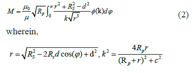
In this paper we use the general formula for calculating the mutual inductance between two circular loops with angular misalignment, whose axes intersect but not at the center either of one, to calculate the restoring and the repulsive magnetic force between them (Figure 1) [1].


Figure 1: Filamentary circular loops with angular misalignment (axes intersect but not at the center either of one).
Rp and Rs are the radii of the primary and secondary loops in (m), respectively.
d-is the perpendicular distance between the axes of coils in (m).
c-is the axial distance between the centers of coils in (m).
θ-is angle in radian, between unit vector normal of the inclined loop positioned at its center and the unit vector of the axis z of the primary loop.
μ0=4��.10-7H/m is the permeability of vacuum.
In (1) angle θ takes the value 0 ≤ θ ≤ ��/2.
In Song et al., gave the modified Grover’s formula (1) (when θ=0), for calculating the mutual inductance between two non-coaxial loops with the parallel axes [15,16].
The restoring (radial) and the repulsive (axial) magnetic force can be obtained by [3],
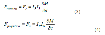
According the force between two filaments is one of the attractions if the currents in them are in the same direction around the common axis [1]. If the currents in the two filaments are in opposite directions around the common axis, the force between them is one of repulsion.
Using (2), (3) and (4) we have,
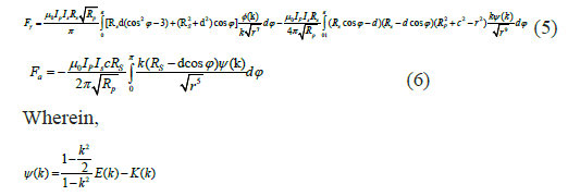
E (k) and K (k) are the complete elliptic function of the first and the second kind [17,18].
Filament method for calculating the magnetic force Fr and Fa between two non-coaxial coils of rectangular cross-section with parallel axes
Let us treat two non-coaxial coils of rectangular cross-section with the parallel axes see (Figure 2).

Figure 2: Configuration of mesh matrix: Two non-coaxial coils of rectangular cross- section with the parallel axes.
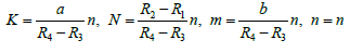
Using the filament method [6], [9] and [12] the formulas for the mutual inductance M as well as for the magnetic forces Fr and Fa are as follows,


I1-Current in the primary coil
I2-Current in the secondary coil
N1-Number of turns in the primary coil
N2-Number of turns in the secondary coil
R1-Inner radius of the primary coil of rectangular cross section
R2-Outer radius of the primary coil of rectangular cross section
R3-Inner radius of the secondary coil of rectangular cross section
R4-Outer radius of the secondary coil of rectangular cross section
a and b-Heights of the primary and the secondary coil, respectively.
d-Perpendicular distance between axes of coils.
c-Distance between the plans of centers of coils.
RP (h)-Average radius of the primary coil positioned in the plane (x, y) whose axis is ‘z’ axis.
RS (l)-Inclined average radius of the secondary coil
K, N, n, and m-The number of the subdivisions of thick coils.
Results and Discussion
Example 1
In this example we calculate the mutual inductance, the restoring and the propulsive magnetic force as a function of the displacement of two non-coaxial loops with the parallel axes where we have: RP =42.5 mm, RS =20 mm. The perpendicular distance between coils axes is d=3 mm, [10].
Clearly, we obtained identical results because the formulas are the same; however, equation (2) is derived without using the angle of inclination. In both cases the single integration is used. The absolute discrepancy AD is zero in each case. Here, we present another numerical approach to solve equation (2), which are particularly interesting from an engineering perspective. Equation (2) is solved using the summation of small segments of the interval over the range (0, ��), thereby avoiding numerical integration. This assumption allows for a considerable reduction in computational time with very high accuracy [5] (Table 1). In Table 2, we provide a comparative calculation of equation (2) using both integration and summation methods (Table 2).
| c (m) | M (nH) | M (nH) | A.D. (%) |
|---|---|---|---|
| 0 | 20.48852432867563 | 20.48852432867563 | 0 |
| 0.001 | 20.46296134770761 | 20.46296134770761 | 0 |
| 0.002 | 20.38668420445834 | 20.38668420445834 | 0 |
| 0.003 | 20.26090954763262 | 20.26090954763262 | 0 |
| 0.004 | 20.08760437072583 | 20.08760437072583 | 0 |
| 0.005 | 19.86940071618871 | 19.86940071618871 | 0 |
| 0.006 | 19.60948700160182 | 19.60948700160182 | 0 |
| 0.007 | 19.31148475780680 | 19.31148475780680 | 0 |
| 0.008 | 18.97931979155518 | 18.97931979155518 | 0 |
| 0.009 | 18,61709599187806 | 18,61709599187806 | 0 |
| 0.01 | 18.22897847733389 | 18.22897847733389 | 0 |
| 0.011 | 17.81909087755921 | 17.81909087755921 | 0 |
Table 1: Mutual inductance as a function of the axial displacement c of two non-coaxial loops with the parallel axes, using single integration [1,2].
| c (m) | M (nH) | M (nH) (2) | A.D. (%) |
|---|---|---|---|
| Single integration | Summation | ||
| 0 | 20.48852432867563 | 20.49048986995235 | 0.00959337649 |
| 0.001 | 20.46296134770761 | 20.46492499834691 | 0.00959612152 |
| 0.002 | 20.38668420445834 | 20.38864220081033 | 0.00960429039 |
| 0.003 | 20.26090954763262 | 20.26285819617522 | 0.00961777425 |
| 0.004 | 20.08760437072583 | 20.08954001265537 | 0.00963600185 |
| 0.005 | 19.86940071618871 | 19.87131994910612 | 0.00965923907 |
| 0.006 | 19.60948700160182 | 19.61138637150371 | 0.00968597445 |
| 0.007 | 19.31148475780680 | 19.31336108410397 | 0.00971611619 |
| 0.008 | 18.97931979155518 | 18.98117010170295 | 0.00974908567 |
| 0.009 | 18,61709599187806 | 18.61891789353698 | 0.00978617535 |
| 0.01 | 18.22897847733389 | 18.23076914790572 | 0.00982320854 |
| 0.011 | 17.81909087755921 | 17.82084807899210 | 0.00986134166 |
Table 2: Mutual inductance as a function of the axial displacement c of two non-coaxial loops with the parallel axes, using single integration and summation [1,5].
From Table 2 we can see a very good agreement between two numerical approaches with the absolute discrepancy around 0.0097%. For these examples MATLAB is used to calculate numerically the single integral on the interval (0, ��) and FORTRAN is used to calculate the summation of the kernel function on the interval (0, ��).
In Tables 3 and 4 the restoring and the axial forces calculations are given for (5) and (6) are compared with the results obtained in [10]. The single integration is used in (5) and (6). Clearly, we obtained identical results by two approaches.
| c (m) | Restoring force | Restoring force (5) | A.D. (%) |
|---|---|---|---|
| Fr (µ N) | Fr (µN) | ||
| 0 | 0.07547749710028973 | 0.07547749710028973 | 0 |
| 0.001 | 0.07488583327209774 | 0.07488583327209774 | 0 |
| 0.002 | 0.07313671349198709 | 0.07313671349198709 | 0 |
| 0.003 | 0.07030546181947066 | 0.07030546181947066 | 0 |
| 0.004 | 0.06651032498899204 | 0.06651032498899204 | 0 |
| 0.005 | 0.06190265669550978 | 0.06190265669550978 | 0 |
| 0.006 | 0.05665516867960698 | 0.05665516867960698 | 0 |
| 0.007 | 0.05094972551589357 | 0.05094972551589357 | 0 |
| 0.008 | 0.04496601777908185 | 0.04496601777908185 | 0 |
| 0.009 | 0.03887211239892259 | 0.03887211239892259 | 0 |
| 0.01 | 0.03281745285065881 | 0.03281745285065881 | 0 |
| 0.011 | 0.02692846490789022 | 0.02692846490789022 | 0 |
Table 3: Restoring force as a function of the axial displacement c of two non-coaxial loops with the parallel axes, using single integration [10].
| c (m) | Repulsive force | Repulsive force (6) | A.D. (%) |
|---|---|---|---|
| Fa (µ N) | Fa (µN) | ||
| 0 | 0.00 | 0.00 | 0 |
| 0.001 | -0.0510570118824195 | -0.0510570118824195 | 0 |
| 0.002 | -0.1012935792952149 | -0.1012935792952149 | 0 |
| 0.003 | -0.1499264624141375 | -0.1499264624141375 | 0 |
| 0.004 | -0.1962433850245375 | -0.1962433850245375 | 0 |
| 0.005 | -0.2396304448823946 | -0.2396304448823946 | 0 |
| 0.006 | -0.2795912286657358 | -0.2795912286657358 | 0 |
| 0.007 | -0.3157568384768270 | -0.3157568384768270 | 0 |
| 0.008 | -0.3478871535458957 | -0.3478871535458957 | 0 |
| 0.009 | -0.3758645407463232 | -0.3758645407463232 | 0 |
| 0.01 | -0.3996817851575968 | -0.3996817851575968 | 0 |
| 0.011 | -0.4194262218421366 | -0.4194262218421366 | 0 |
Table 4: Repulsive force as a function of the axial displacement c of two non-coaxial loops with the parallel axes, using single integration [10].
Here, we present another numerical approach to solve equations (5) and (6), which are particularly interesting from an engineering perspective. Equations (5) and (6) are solved using the summation of small intervals over the range (0, ��), thereby avoiding numerical integration. This assumption allows for a considerable reduction in computational time with very high accuracy. In Tables 5 and 6, we provide a comparative calculation of equations (5) and (6) using both integration and summation methods [5].
| c (m) | Restoring force (5) | Restoring force (5) | A.D. (%) |
|---|---|---|---|
| Fr (µN) Single integral | Fr (µN) Summation | ||
| 0 | 0.07547749710028973 | 0.07525745846863121 | 0.29 |
| 0.001 | 0.07488583327209774 | 0.07466619941804611 | 0.29 |
| 0.002 | 0.07313671349198709 | 0.07291828457836584 | 0.3 |
| 0.003 | 0.07030546181947066 | 0.07008901078750480 | 0.3 |
| 0.004 | 0.06651032498899204 | 0.06629657942474166 | 0.32 |
| 0.005 | 0.06190265669550978 | 0.06169228882577443 | 0.34 |
| 0.006 | 0.05665516867960698 | 0.05644877724710618 | 0.36 |
| 0.007 | 0.05094972551589357 | 0.05074783460471877 | 0.4 |
| 0.008 | 0.04496601777908185 | 0.04476907078064662 | 0.44 |
| 0.009 | 0.03887211239892259 | 0.03868047679800412 | 0.49 |
| 0.01 | 0.03281745285065881 | 0.03263140496709844 | 0.57 |
| 0.011 | 0.02692846490789022 | 0.02674821108617715 | 0.67 |
Table 5: Restoring force as a function of the axial displacement c of two non-coaxial loops with the parallel axes, using single integration and summation [1,5].
| c (m) | Repulsive force (6) | Repulsive force (6) | A.D. (%) |
|---|---|---|---|
| Fa (µN) Single integral | Fa (µN) Summation | ||
| 0 | 0.00 | 0.00 | -- |
| 0.001 | -0.0510570118824195 | -0.0510607877912594 | 0.0074 |
| 0.002 | -0.1012935792952149 | -0.1013010959350985 | 0.0074 |
| 0.003 | -0.1499264624141375 | -0.1499376442971153 | 0.0075 |
| 0.004 | -0.1962433850245375 | -0.1962581393878131 | 0.0075 |
| 0.005 | -0.2396304448823946 | -0.2396486153037206 | 0.0076 |
| 0.006 | -0.2795912286657358 | -0.2796126687702186 | 0.0077 |
| 0.007 | -0.3157568384768270 | -0.3157813532493243 | 0.0078 |
| 0.008 | -0.3478871535458957 | -0.347914523854540 | 0.0079 |
| 0.009 | -0.3758645407463232 | -0.3758945034502981 | 0.008 |
| 0.010 | -0.3996817851575968 | -0.3997141139905325 | 0.0081 |
| 0.011 | -0.4194262218421366 | -0.4194606522115783 | 0.0082 |
Table 6: Repulsive force as a function of the axial displacement c of two non-coaxial loops with the parallel axes, using single integration and summation.
The results of the restoring and repulsive forces using the numerical integration (MATLAB) and the summation (FORTRAN) are given in Tables 5 and 6. All results are in very good agreement either by the numerical integration or the numerical summation. The average absolute discrepancy is about 0.0097%.
Example 2
Parameters for two non-coaxial cylindrical coils with parallel axes given in are as follows [13]:

Here, we will calculate the mutual inductance by the presenting method using the filament method using the same and different numbers of the subdivisions. Our goal is to find the best accuracy and the smallest computational time if possible.
Let us begin with the same number of the subdivisions K=N=m=n=20.
It is obvious from Table 7 that results obtained by two different approaches are in very good agreement with the absolute average discrepancy about 0.0075%, but the computational time for the filament method is considerably enormous.
Preferable from the engineering point of consideration thus, the same number of subdivisions is not the smart choice in the mutual inductance calculation using the filament method. We can have very good precision of obtained results but with considerably big computational tame. This is why one must find the good compromise between the accuracy and the computational time in the choice of the number of the subdivisions of coils.
| d (m) | M (mH) | M (mH), (7) | Time (s) | A.D. (%) |
|---|---|---|---|---|
| 0.000 | 56.89550827752887 | 56.89876728224178 | 856.952685 | 0.0057 |
| 0.003 | 56.91083176832369 | 56.91408965245684 | 867.414842 | 0.0057 |
| 0.005 | 56.93806682400835 | 56.94132270480409 | 2761.818773 | 0.0057 |
| 0.008 | 57.00441609146245 | 57.00766703064307 | 1177.523890 | 0.0057 |
| 0.011 | 57.10129482231152 | 57.10453856704491 | 521.859077 | 0.0057 |
| 0.224 | −5.774844679019263 | -5.775269172262961 | 419.295176 | 0.007 |
| 0.250 | −4.026004905310310 | -4.026291199492929 | 452.488898 | 0.007 |
| 0.300 | −2.194029475697561 | -2.194140166466710 | 361.227363 | 0.005 |
| 0.400 | −0.8609762300871849 | -0.860995852556949 | 505.658034 | 0.002 |
| 0.500 | −0.4256179797832593 | -0.425622573906044 | 1648.168221 | 0.001 |
Table 7: Mutual inductance as a function of the perpendicular displacement d [13].
Now, let’s conduct the following analysis concerning the coil dimensions and the number of subdivisions. We propose the optimization method to minimize the three subdivisions (variables) in the function of one subdivision (variable) for the given coils’ dimensions. The relations between two subdivisions are linear. It means that we have the problems of four linear homogenic equations where one depends on the others three. We use the following reasoning to find the minimal number of the subdivisions (variables) to reduce the computational time end keep the good accuracy. Choosing the smallest dimension between the radial and axial coils dimensions (LN=R2-R1, Ln=R4-R3, La=z2-z1=a, Lb=z4-z3=b), we arbitrary choose the corresponding subdivision. Other three subdivisions will depend on this arbitrarily chosen subdivision. The procedures are as follows:
Find t=min {LN, La, Ln, Lb} = tmin
For obtained tmin, we choose the corresponding variable (subdivision), for example n→ tmin.
In this example we have,
R2-R1=4.15485; R4-R3=1.397; a=2.413; b=14.2748. The smallest dimension is R4-R3=1.397 which corresponds to the radial subdivision n of the second coil. Let us expresses all subdivisions in the function of n.
N/n = ((R2-R1) / (R4-R3)) = (2.9727) = 3 or N=3n K/n = (a / (R4-R3)) = (1.72727) = 2 or K=2n m/n = (b / (R4-R3)) = (10.218218) = 10 or m=10n
In the Tables 8-10 we give the calculations of the mutual inductance by the filament method where the values of n subdivisions are different. All other subdivisions K, N and m are in the function of n as previously discussed.
| d (m) | M (mH) | M (mH), (7) | Time (s) | A.D. (%) |
|---|---|---|---|---|
| 0 | 56.89550827752887 | 56.89286673907408 | 11.337791 | 0.0046 |
| 0.003 | 56.91083176832369 | 56.90818957928507 | 10.567271 | 0.0046 |
| 0.005 | 56.93806682400835 | 56.93542347847519 | 10.742036 | 0.0046 |
| 0.008 | 57.00441609146245 | 57.00176992753069 | 10.759457 | 0.0046 |
| 0.011 | 57.10129482231152 | 57.09864457245561 | 10.969503 | 0.0046 |
| 0.224 | −5.774844679019263 | -5.774288816171031 | 11.535825 | 0.0096 |
| 0.250 | −4.026004905310310 | -4.025622477401055 | 10.564258 | 0.0095 |
| 0.300 | −2.194029475697561 | -2.193828394461475 | 10.826811 | 0.0092 |
| 0.400 | −0.8609762300871849 | -0.860900867409665 | 10.847333 | 0.0088 |
| 0.500 | −0.4256179797832593 | -0.425581528154343 | 10.518138 | 0.0086 |
Table 8: Mutual inductance as a function of the perpendicular displacement d [13].
| d (m) | M (mH) | M (mH), (7) | Time (s) | A.D. (%) |
|---|---|---|---|---|
| 0 | 56.89550827752887 | 56.89385079631084 | 30.964315 | 0.003 |
| 0.003 | 56.91083176832369 | 56.90917390279342 | 31.016049 | 0.003 |
| 0.005 | 56.93806682400835 | 56.93640827549144 | 31.642019 | 0.003 |
| 0.008 | 57.00441609146245 | 57.00275587942618 | 35.509275 | 0.003 |
| 0.011 | 57.10129482231152 | 57.09963217765802 | 93.66061 | 0.003 |
| 0.224 | -5.774844679019263 | -5.774507929355869 | 115.902304 | 0.006 |
| 0.250 | -4.026004905310310 | -4.025773287164149 | 161.774595 | 0.006 |
| 0.300 | -2.194029475697561 | -2.193908170034211 | 126.383069 | 0.006 |
| 0.400 | -0.8609762300871849 | -0.860931031003053 | 114.444533 | 0.005 |
| 0.500 | -0.4256179797832593 | -0.42559617669354 | 151.118313 | 0.005 |
Table 9: Mutual inductance as a function of the perpendicular displacement d [13].
| d (m) | M (mH) | M (mH), (7) | Time (s) | A.D. (%) |
|---|---|---|---|---|
| 0 | 56.89550827752887 | 56.8943751557484 | 194.760392 | 0.002 |
| 0.003 | 56.91083176832369 | 56.9096983928553 | 72.493173 | 0.002 |
| 0.005 | 56.93806682400835 | 56.93693299776592 | 122.589127 | 0.002 |
| 0.008 | 57.00441609146245 | 57.00328116767053 | 132.458158 | 0.002 |
| 0.011 | 57.10129482231152 | 57.10015829724649 | 152.743919 | 0.002 |
| 0.224 | -5.774844679019263 | -5.774619127636496 | 265.588813 | 0.004 |
| 0.250 | -4.026004905310310 | -4.025849785469264 | 309.18101 | 0.004 |
| 0.300 | -2.194029475697561 | -2.193948422607928 | 128.801917 | 0.004 |
| 0.400 | -0.8609762300871849 | -0.860946133501390 | 285.441115 | 0.0035 |
| 0.500 | -0.4256179797832593 | -0.425603088258163 | 401.471515 | 0.0035 |
Table 10: Mutual inductance as a function of the perpendicular displacement d [13].
From Tables 8-10 we can see very good agreement between two approaches. In all calculations we have very high accuracy between two different approaches where the average absolute discrepancy is about 0.0069%, (Table 8), 0.0043%, (Table 9) and 0.0029%, (Table 10). Also, for both methods we have for each calculation the same four significant figures. Moreover, the calculation for the different number of the subdivisions considerably reduced the computational time (Tables 7 and 9) regarding the calculation for the same number of the subdivisions (Table 7).
Even though there is not considerable difference between the calculations regarding the accuracy given in Tables 7 and 9, it is recommended to choose K=6, N=9, m=30 and n=3. Also, without any reserve one can take K=8, N=12, m=40 and n=4, because of a very good accuracy and the relatively small computational time.
In Table 8 we choose n=3, that gives K=6, N=9 and m=30. In Table 9 we choose n=4, that gives K=8, n=4, N=12 and m=40. In Table 10 we choose n=5, that gives K=10, N=15 and m=50.
Also, we give the mutual inductance calculation obtained by the summation, Table 9. These results are expected regarding the accuracy and the computational time because we used the summation instead the integration [1,5]. The number of the subdivisions is K=N=m=n=20. These results are in the good agreement with those obtained by two previous methods.
In the calculations of the restoring (radial) and the repulsive (axial) forces we will use the same reasoning in the choice of the number of the subdivisions.
Example 3
From Example 2, let’s calculate the restoring and repulsive magnetic forces between the coils in questions. Here, we utilize the optimal choice of subdivisions, with ��=8, ��=12, ��=40, and ��=4, as determined in the previous example. This selection ensures both good accuracy and minimal computational time for the integral approach. In contrast, for the summation approach, the number of subdivisions is set to ��=��=��=��=20.
The comparison will involve using the formulas (8) for the radial magnetic force and (9) for the axial magnetic force, obtained through integration (as presented in this work), alongside the method that employs summation instead of integration, as outlined in reference [5].
From Tables 11 and 12 we have the good agreement between results obtained two methods in which the numerical integration and the numerical summation are used on the interval of the consideration . Obviously that the results for the radial magnetic force Fr, (8) obtained by the numerical integration are more precise, but the method is usable as comparative benchmark. The absolute discrepancy is between 0.1% and 1.06% [1,5].
| d (m) | M (mH) | M (mH) | Time (s) | A.D. (%) |
|---|---|---|---|---|
| 0 | 56.89550827752887 | 56.88331624723717 | 36 | 0.0214 |
| 0.003 | 56.91083176832369 | 56.89896818427943 | 37 | 0.0208 |
| 0.005 | 56.93806682400835 | 56.92641707644633 | 37 | 0.0205 |
| 0.008 | 57.00441609146245 | 56.99307960663946 | 37 | 0.0199 |
| 0.011 | 57.10129482231152 | 57.09026280933549 | 37 | 0.0193 |
| 0.224 | -5.774844679019263 | -5.764590879596135 | 37 | 0.178 |
| 0.250 | -4.026004905310310 | -4.018716712530881 | 36 | 0.181 |
| 0.300 | -2.194029475697561 | -2.189813740930188 | 36 | 0.192 |
| 0.400 | -0.8609762300871849 | -0.859076834887261 | 36 | 0.220 |
| 0.500 | -0.4256179797832593 | -0.424546874039815 | 36 | 0.251 |
Table 11: Mutual inductance as a function of the perpendicular displacement d, using the summation [5,13].
| d (m) | Fr (mN), (8) | Fr (mN), (8) | A.D. (%) |
|---|---|---|---|
| 0 | -3.494310397 e-14~ 0 | 0.111041384395338 | -- |
| 0.003 | 10.21401930788771 | 10.32269230189135 | 1.06 |
| 0.005 | 17.01798782490178 | 17.12512978277371 | 0.63 |
| 0.008 | 27.20764213665493 | 27.31257183181061 | 0.39 |
| 0.011 | 37.36736781567217 | 37.47032614951112 | 0.28 |
| 0.224 | 83.08829769865285 | 82.94606120526218 | 0.17 |
| 0.250 | 53.55797101390077 | 53.46734216052616 | 0.17 |
| 0.300 | 24.21219509927497 | 24.17102394119574 | 0.17 |
| 0.400 | 6.873995953355325 | 6.861513422034208 | 0.18 |
| 0.500 | 2.660323169441172 | 2.655031212570641 | 0.2 |
Table 12: The radial magnetic force as a function of the perpendicular displacement d. using the numerical integration [1] and the summation [3].
From Table 13 the axial magnetic force Fa is zero for all points of the calculation that is practically confirmed by the presented method, equation (9). The second method doesn’t give exactly zero for the axial force Fa because of the positive and negative variations during the summation on the interval of the consideration. The third method give exactly zero due to the axial factor involved in the force expression [5,15].
| d (m) | Fa (mN) (9) | Fa (mN)(9) |
|---|---|---|
| 0 | 4.7457265094e-15~ 0 | 0 |
| 0.003 | 8.4129547976e-16~ 0 | 0 |
| 0.005 | -2.2009000655e-15~ 0 | 0 |
| 0.008 | -6.3471089636e-16~ 0 | 0 |
| 0.011 | 6.4183753659e-16 ~ 0 | 0 |
| 0.224 | -4.2605870746e-17~ 0 | 0 |
| 0.25 | 1.6914772640e-16~ 0 | 0 |
| 0.3 | 8.0537633318e-17~ 0 | 0 |
| 0.4 | 2.5785955007e-17~ 0 | 0 |
| 0.5 | 1.0128379992e-18~ 0 | 0 |
Table 13: The axial magnetic force as a function of the perpendicular displacement d. using the numerical integration and the summation [1,3 ,5,15].
where h1=a/2 and h2=b/2, and κ are the eigenvalues due to the introduction of artificial boundary, and it can be concluded that Fa=0 from f2(κ, 0) = 0.
Example 5
Here, we give this example that can be used as the benchmark problem for tasting the different methods that treat the coils in question.
Parameters for two non-coaxial cylindrical coils with parallel axes given in [6] and used in [14] are as follows:

Let us find the following values.
LN=R2-R1=0.01397, Ln=R4-R3=0.041529,
La=z2-z1=a=0.142748, Lb=z4-z3=b=0.02413
A) Let us find the minimum values between them.
t=min {LN, La, Ln, Lb} = LN=tmin=0.01397
B) This minimum value must correspond to following variable (subdivision).
tmin=0.01397→N
C) Three variables (subdivisions) in the function of this variable are as follows:
K = (a / (R2-R1)) N = (10.218181) = 10 or K=10N m/N = (b / (R2-R1)) = (1.72727) = 2 or m=2N n/N=((R4-R3) / (R2-R1)) = (2.9727) = 3 or n=3N
D) The next step is to find the best choice of subdivisions for the arbitrarily chosen smallest variable.
In Table 14, for one calculation of the mutual inductance given in [13], with d=0.006 m, c=0.059309 m, M=44.7454180199 mH, we test different values of N = {1,2,3,4,5,6,7,8}.
| K/N/m/n | M (mH), (7) | Time (s) | A.D. (%) |
|---|---|---|---|
| 10/1/2/3 | 44.73698768471552 | 0.724790 | 0.01884 |
| 20/ 2/4/6 | 44.74148468303699 | 4.277472 | 0.00879 |
| 30/ 3/6/9 | 44.74326891694706 | 11.439728 | 0.0048 |
| 40/4/8/12 | 44.74407612900293 | 36.149399 | 0.00300 |
| 50/5/10/15 | 44.74450319954718 | 218.047730 | 0.00204 |
| 60/6/12/18 | 44.74475522011805 | 145.106737 | 0.00148 |
| 70/7/14/21 | 44.74491602293224 | 873.712863 | 0.00112 |
| 80/8/16/23 | 44.74502477488414 | 3226.565 | 0.00088 |
Table 14: The best choice of the number of the subdivisions.
Obviously, it is not logical to increase the number of subdivision N beyond 4 because the accuracy doesn’t change significantly while the computational time increases enormously. Moreover, it is not practical from the engineering point of view. Thus, the best choice is to take N=3 or even N=4.
We can further improve the accuracy and computational time of calculations by adjusting the number of subdivisions based on our previous choices. By minimizing a chosen subdivision (variable), we then select the next smaller dimension with a corresponding subdivision (variable).
These two subdivisions may be increased by 1, 2, or 3, while the other two are decreased by 1, 2 or 3. This approach can significantly improve both accuracy and computational time.
From the previous Table 14 we begin with the choice of N=3. Now, K1=30, N1=3, m1=6, N1=9.
The following calculation will increase two the two smallest variables by 1 and decrease the two largest variables by 1, Table 15. This process can be continued using the same logic, successively incrementing, and decrementing the variables by 1. This means K2=29, N2=4, m2=7, N2=8 and so on.
| K1/N1/m1/n1 | M (mH), (7) | Time (s) | A.D. (%) |
|---|---|---|---|
| 30/ 3/6/9 | 44.74326891694706 | 11.439728 | 0.0048 |
| 29/4/7/8 | 44.74436616452383 | 14.218988 | 0.0024 |
| 28/5/8/7 | 44.74479926514896 | 16.099376 | 0.0014 |
| 27/6/9/6 | 44.74487932957280 | 18.593136 | 0.0012 |
| 26/7/10/5 | 44.74465342835332 | 19.083521 | 0.0017 |
Table 15: The best choice of the number of the subdivisions.
From Table 15, one can see that the previous statement is effective, as the accuracy does not change significantly and neither does the computational time.
Practically, we proposed a new approach in choosing the optimal numbers for the variables (subdivisions) that archives very high accuracy and the smallest possible time of calculation.
Let us choose N=3, that gives,
K=30; N=3; m=6; n=9.
Now, we calculate by the presented method the mutual inductance given [14] and test the computational time and the accuracy. All comparative results are given in Table 16.
| d (m) | c (m) | M | M, (7) | Time (s) | A.D (%) |
|---|---|---|---|---|---|
| 0.006 | 0.01 | 56.6162643374 | 56.61363465455378 | 50.949498 | 0.0046 |
| 0.006 | 0.02 | 55.5894956502 | 55.5869094089611 | 51.984518 | 0.0047 |
| 0.006 | 0.03 | 53.8629343708 | 53.86042062215667 | 22.085411 | 0.0047 |
| 0.006 | 0.04 | 51.4222297882 | 51.41981711532675 | 17.279959 | 0.0047 |
| 0.006 | 0.05 | 48.2700337321 | 48.26774838654966 | 18.802184 | 0.0047 |
| 0.006 | 0.059309 | 44.7454180199 | 44.74326891694706 | 11.439728 | 0.0048 |
| 0.006 | 0.07 | 40.1814759728 | 40.17949410516751 | 10.649205 | 0.0049 |
| 0.006 | 0.083439 | 34.2304828323 | 34.22872135097286 | 22.910502 | 0.0051 |
| 0.006 | 0.09 | 31.4566003446 | 31.45494874434184 | 31.219811 | 0.0053 |
| 0.006 | 0.1 | 27.5571415229 | 27.55565306023951 | 22.247917 | 0.0054 |
| 0.006 | 0.6 | 0.4370202882 | 0.4369853665835998 | 21.303489 | 0.008 |
| 0.006 | 1 | 0.0979060786 | 0.09789809468339546 | 15.960037 | 0.0082 |
| 0.020 | 0.083439 | 33.9467350341 | 33.94496955449947 | 22.260440 | 0.0052 |
| 0.020 | 0.09 | 31.0753970232 | 31.07375095703897 | 17.657343 | 0.0053 |
| 0.020 | 0.1 | 27.1316988802 | 27.13022256109052 | 18.291836 | 0.0054 |
| 0.020 | 0.6 | 0.4358068619 | 0.4357720325526511 | 16.392457 | 0.008 |
| 0.020 | 1 | 0.0978025141 | 0.09779453844705811 | 37.723350 | 0.0082 |
| 0.250 | 0.01 | -3.9917061128 | -3.991327116889206 | 17.017424 | 0.0095 |
| 0.250 | 0.02 | -3.8892645048 | -3.888895853203926 | 17.197398 | 0.0095 |
| 0.250 | 0.03 | -3.7202594312 | -3.719908143385208 | 22.417223 | 0.0094 |
| 0.250 | 0.04 | -3.4880421240 | -3.487715260454917 | 22.161433 | 0.0094 |
| 0.250 | 0.05 | -3.1987715126 | -3.198475841930457 | 16.959263 | 0.0092 |
| 0.250 | 0.059309 | -2.8870312678 | -2.8867700832056 | 17.120941 | 0.009 |
| 0.250 | 0.07 | -2.4940353652 | -2.493817639836896 | 18.719902 | 0.0087 |
| 0.250 | 0.083439 | -1.9793349081 | -1.979173375602797 | 18.864897 | 0.0082 |
| 0.250 | 0.09 | -1.7317005825 | -1.731565514863421 | 18.237672 | 0.0078 |
| 0.250 | 0.1 | -1.3709099874 | -1.370811777058473 | 10.940643 | 0.0072 |
| 0.250 | 0.6 | 0.2768190451 | 0.2767965107849468 | 10.749782 | 0.0081 |
| 0.250 | 1 | 0.0819441585 | 0.08193745655136937 | 11.089051 | 0.0082 |
Table 16: Mutual inductance M(mH) as a function of the perpendicular displacement d [14].
For the previously chosen the number of subdivisions, K=30; N=3; m=6; n=9, we calculate the radial and the axial magnetic force between the coils in questions. The method given in [15,16] is used as the comparative method. The calculation of Fr and Fa can be used as the benchmark problem for tasting other methods for calculating these two magnetic forces for coils in question regarding the accuracy and the computational time.
From Tables 17 and 18 one can see very good agreements of results obtained by two different methods even though there are some differences for some points of the calculations. It can be explained by the following facts.
| d (m) | c (m) | Fr, (8) | Fr |
|---|---|---|---|
| 0.006 | 0.01 | 20.576008 | 20.602994 |
| 0.006 | 0.02 | 20.9902 | 21.039176 |
| 0.006 | 0.03 | 21.439313 | 21.54829 |
| 0.006 | 0.04 | 21.400845 | 21.663334 |
| 0.006 | 0.05 | 19.748335 | 19.744878 |
| 0.006 | 0.059309 | 15.02043 | 15.057457 |
| 0.006 | 0.07 | 4.9434673 | 5.075121 |
| 0.006 | 0.083439 | -7.967173 | -7.932075 |
| 0.006 | 0.09 | -11.538574 | -11.626505 |
| 0.006 | 0.1 | -13.554995 | -13.571601 |
| 0.006 | 0.6 | -0.040067 | -0.042237 |
| 0.006 | 1 | -0.003416 | -0.003751 |
| 0.020 | 0.083439 | -36.535795 | -36.780664 |
| 0.020 | 0.09 | -45.290737 | -45.297743 |
| 0.020 | 0.1 | -48.219792 | -48.217222 |
| 0.020 | 0.6 | -0.133111 | -0.135434 |
| 0.020 | 1 | -0.011372 | -0.012146 |
| 0.250 | 0.01 | 52.955752 | 52.724566 |
| 0.250 | 0.02 | 51.142662 | 51.096883 |
| 0.250 | 0.03 | 48.047731 | 47.986993 |
| 0.250 | 0.04 | 43.5982 | 43.504992 |
| 0.250 | 0.05 | 37.78111 | 37.632765 |
| 0.250 | 0.059309 | 31.269094 | 31.279649 |
| 0.250 | 0.07 | 22.934243 | 22.893013 |
| 0.250 | 0.083439 | 12.369791 | 12.358394 |
| 0.250 | 0.09 | 7.635737 | 7.67972 |
| 0.250 | 0.1 | 1.330825 | 1.330104 |
| 0.250 | 0.6 | -0.970102 | -0.971188 |
| 0.250 | 1 | -0.114421 | -0.115135 |
Table 17: Radial magnetic force Fr (mN) as a function of the perpendicular displacement d [14-16].
| d (m) | c (m) | Fa, (9) | Fa |
|---|---|---|---|
| 0.006 | 0.01 | -68.191312 | -68.205467 |
| 0.006 | 0.02 | -137.391008 | -137.389334 |
| 0.006 | 0.03 | -208.17323 | -208.158349 |
| 0.006 | 0.04 | -279.963203 | -279.898948 |
| 0.006 | 0.05 | -349.604001 | -349.520901 |
| 0.006 | 0.059309 | -405.214825 | -405.294053 |
| 0.006 | 0.07 | -442.39077 | -442.207026 |
| 0.006 | 0.083439 | -433.226828 | -433.30756 |
| 0.006 | 0.09 | -411.017469 | -411.060773 |
| 0.006 | 0.1 | -367.800478 | -367.886034 |
| 0.006 | 0.6 | -2.102442 | -2.102696 |
| 0.006 | 1 | -0.289647 | -0.28981 |
| 0.02 | 0.083439 | -454.238985 | -454.305635 |
| 0.02 | 0.09 | -420.626836 | -420.633025 |
| 0.02 | 0.1 | -368.311148 | -368.32578 |
| 0.02 | 0.6 | -2.092916 | -2.093189 |
| 0.02 | 1 | -0.28914 | -0.289332 |
| 0.25 | 0.01 | 6.851848 | 6.851354 |
| 0.25 | 0.02 | 13.609163 | 13.606354 |
| 0.25 | 0.03 | 20.134301 | 20.13318 |
| 0.25 | 0.04 | 26.203735 | 26.196089 |
| 0.25 | 0.05 | 31.476643 | 31.448595 |
| 0.25 | 0.059309 | 35.281758 | 35.276902 |
| 0.25 | 0.07 | 37.883856 | 37.88465 |
| 0.25 | 0.083439 | 38.163078 | 38.169832 |
| 0.25 | 0.09 | 37.213046 | 37.211353 |
| 0.25 | 0.1 | 34.771519 | 34.77153 |
| 0.25 | 0.6 | -0.958292 | -0.958551 |
| 0.25 | 1 | -0.214685 | -0.214975 |
Table 18: Axial magnetic force Fa (mN) as a function of the perpendicular displacement d [14-16].
1. The presented method treats two coils of rectangular crosssection with the parallel axes, in the unbounded space libre, which are divided into circular filamentary coils. To account for the finite dimensions of the coils, massive solenoids are subdivided into meshes of filamentary coils as shown at Figure 2. The cross-sectional areas of two coils are divided into (2K+1) by (2N+1) cells for the first coil and (2m+1) by (2n+1) cells for the second coil, where K, N, m and n are the numbers of the subdivisions of coils [6,9,12]. Even though we use the analytical Maxwell’s formulas for the mutual inductance or the magnetic force between two circular loops, we cannot say that the presented filament method for the massive coils is purely analytical because its precision and the computational time depend on the number of subdivisions. This statement was studded in the previous examples. As it was shown the number of the subdivisions has the influence on the accuracy.
2. The compared method is a boundary value problem of circular coils with parallel axes shielded by a cuboid of high permeability. It means the coils are bounded by the medium of high permeability regarding the free space, in which are coils, where the mixed boundary conditions are satisfied on six surfaces of the artificial cuboid. Thus, this approach is approximate, but it proves to be accurate and efficient enough for practical applications. It means that this method can bring some differences in accuracy.
Even though we compare the results obtained by two different methods one for open space and other for artificial boundaries in bounded space, both gives very satisfactory results for calculating the magnetic force between two coils of rectangular cross section with the parallel axes.
With 1) and 2) we explain the possible differences of accuracy for some cases of calculation.
Example 5
Finally, we give the rare examples that can find in the literature to calculate the mutual inductance between two non-coaxial coils of the rectangular cross-section with the parallel axes [1]. For this combination, the dimensions and the number of turns are as follows:
R1=4 cm, R2=6 cm, z2-z1=a=10 cm, N1=150
R3=2.5 cm, R4=3.5 cm, z4-z3=b=5 cm, N1=50
The perpendicular displacement of two coil axes is d=10 cm, and the axial displacement of the centers of the two coils is c=10.5 cm.
In the mutual inductance is [1],
M=3.144 μH
According to the optimal minimizing method given by presented approach concerning the high accuracy and the small computational time, after some tests we choose the number of the subdivisions K=30; N=6; m=15 for arbitrarily chosen n=9.
Using the approach presented in this paper the mutual inductance is,
M=3.13606092090 μH
Elapsed time is 17.133452 seconds (with MATLAB, Intel Core i5-12500H @2.5 GHz).
The method of [15,16] gives,
M=3.136970 μH
and the elapsed time is 5.2 seconds (with Mathematica, Intel Core i7-8700 @3.2 GHz).
The absolute discrepancy regarding the accuracy between the presented method and this one given in [15,16] is around 0.029%.
In the mutual inductance is calculated using the general formula
of Dwight an Purssell, arranged as series involving zonal harmonics,
Equations (190) and (191) [1]. The convergence of this series is sufficient for most purposes as long as all distances  are greater than (A+a), where dm, ρ are the perpendicular displacement
of two coil axes the axial displacement of the centers of the two coils,
respectively. A and a are the mean radii of two coils of rectangular
cross section respectively, [1]. Since the general term of the series
is known, it should be possible to use over the full range. However,
the calculation of higher power terms becomes very tedious and time
consuming [1]. This is why Grower took only four terms of this series
and obtained M=3.144 μH. It was problematic to take more terms
because of mentioned issues as well as very slow convergence [1].
are greater than (A+a), where dm, ρ are the perpendicular displacement
of two coil axes the axial displacement of the centers of the two coils,
respectively. A and a are the mean radii of two coils of rectangular
cross section respectively, [1]. Since the general term of the series
is known, it should be possible to use over the full range. However,
the calculation of higher power terms becomes very tedious and time
consuming [1]. This is why Grower took only four terms of this series
and obtained M=3.144 μH. It was problematic to take more terms
because of mentioned issues as well as very slow convergence [1].
We did many tests of (190) and (191) from which we found very slow convergence. For two terms more we obtain
M=3.14454842613μH
The absolute discrepancy is 0.27%. Taking still more terms which signs changes alternatively will oscillate without significantly improve the accuracy because of the slow convergence.
However, for the different coils dimensions these formulas are not working correctly that is mentioned in [1]. This is why we consider the approach presented here as general for any coil’s dimensions.
Now, let us calculate the radial and the axial magnetic force between the coils in questions respecting all parameters in the previously calculated mutual inductance.
Fr=-136.725877825 μN
Fa=39.3340997099 μN
As a comparison, the method of [15,16] gives,
Fr=-136.753948 μN
Fa=39.344618 μN
Obviously, all results are in very good agreement.
The calculation provided by the presented method could also serve as a benchmark for other methods addressing this problem. Additionally, this method could be automatically applied to calculate the mutual inductance and the magnetic force between other coil configurations (solenoids, disks) with parallel axes.
Conclusion
In this paper we give the new formulas for calculating the restoring (radial) and the repulsive (axial) magnetic forces between two non-coaxial coils of rectangular cross-section with the parallel axes. These formulas are derived from modified Grover’s formula for the mutual inductance between two non-coaxial loops with parallel axes. The validity of the presented approach is validated with an already established method. Presented formulas are used for calculating the radial and the axial force between two non-coaxial coils of rectangular cross-section with parallel axes using the filament method. Also, we presented the method to minimize the variables (subdivisions) in the filament method to find the compromise between the satisfactory accuracy and the corresponding small time of the calculation. We mention this method is applicable between non-coaxial conventional coils with parallel axes (massive-loop; massive-disk; massive-solenoid; two disks; disk-loop; disk-solenoid; two solenoids and solenoid-loop). This method can be useful for the engineers which are working in this domain because of its simplicity. The proposed method is comprehensible, fast, and very precise.
References
- Grover FW (2024) Inductance calculations: Working formulas and tables. Dover Publications.
- Dwight HB (1945) Electrical coils and conductors: Their electrical characteristics and theory. McGraw-Hill Book Company.
- Butterworth S (1916) LIII. On the coefficients of mutual induction of eccentric coils. The London Edinburgh Philos Mag & J Sci 31(185):443-454.
- Snow C (1954) Formulas for computing capacitance and inductance. US Government Printing Office.
- Song KH, Feng J, Zhao R, Wu XL (2019) A general mutual inductance formula for parallel non-coaxial circular coils. Appl Comput Electromagn Soc J (ACES) 1:1385-1390.
- Conway JT (2007) Inductance calculations for noncoaxial coils using bessel functions. IEEE Trans Magn 43(3):1023-34.
- Conway JT (2008) Noncoaxial inductance calculations without the vector potential for axisymmetric coils and planar coils. IEEE Trans Magn 44(4):453-462.
- Akyel C, Babic S, Mahmoudi MM (2009) Mutual inductance calculation for non-coaxial circular air coils with parallel axes. Prog Electromagn Res 91:287-301.
- Kim KB, Levi E, Zabar Z, Birenbaum L (1997) Mutual inductance of noncoaxial circular coils with constant current density. IEEE Trans Magn 33(5):4303-4309.
- Babic S, Akyel C (2011) Magnetic force between inclined circular filaments placed in any desired position. IEEE Trans Magn 48(1):69-80.
- Babic S, Sirois F, Akyel C (2009) Validity check of mutual inductance formulas for circular filaments with lateral and angular misalignments. Prog Electromagn Res 8:15-26.
- Babic S, Akyel C, Ren Y, Chen W (2012) Magnetic force calculation between circular coils of rectangular cross section with parallel axes for superconducting magnet. Prog Electromagn Res 37:275-88.
- Conway JT (2017) Mutual inductance of thick coils for arbitrary relative orientation and position. Prog Electromagn Res 1388-1395.
- Conway JT (2009) Inductance calculations for circular coils of rectangular cross section and parallel axes using Bessel and Struve functions. IEEE Trans Magn 46(1):75-81.
- Luo Y, Zhu Y, Yu Y, Zhang L (2018) Inductance and force calculations of circular coils with parallel axes shielded by a cuboid of high permeability. IET Electr Power App 12(5):717-727.
- Yang X, Luo Y, Kyrgiazoglou A, Zhou X, Theodoulidis T, et al. (2023) Impedance variation of a reflection probe near the edge of a magnetic metal plate. IEEE Sen J 23(14):15479-88.
- Abramowitz M, Stegun IA (1968) Handbook of mathematical functions with formulas, graphs, and mathematical tables. US Government printing office.
- Gradshteyn IS, Ryzhik IM (2014) Table of integrals, series, and products. Academic press.